7.5: Normal Incidence onto a Perfect Conductor

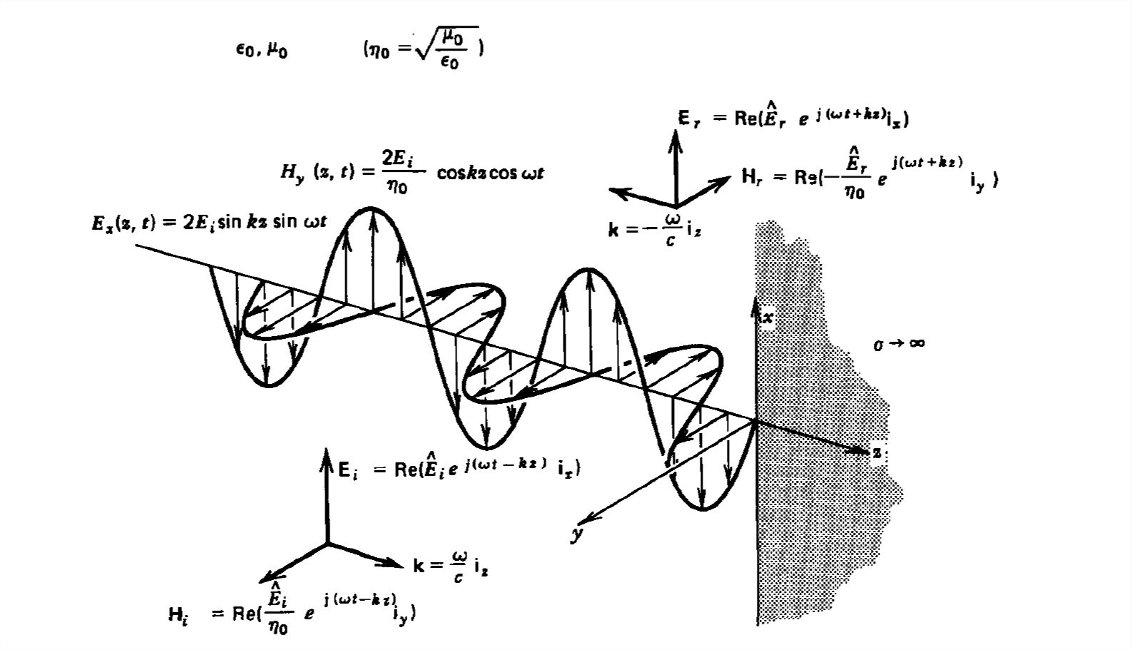
A uniform plane wave with \(x\)-directed electric field is normally incident upon a perfectly conducting plane at \(z =0\), as shown in Figure 7-13. The presence of the boundary gives rise to a reflected wave that propagates in the \(-z\) direction. There are no fields within the perfect conductor. The known incident fields traveling in the \(+z\) direction can be written as

\[ \textbf{E}_{i}\left ( z,t \right )=\textrm{Re}\left ( \hat{E}_{i}e^{j\left ( \omega t-kz \right )}\textbf{i}_{x} \right )\\
\textbf{H}_{i}\left ( z,t \right )=\textrm{Re}\left ( \frac{\hat{E}_{i}}{\eta_{0}}e^{j\left ( \omega t-kz \right )}\textbf{i}_{y} \right )  \]

while the reflected fields propagating in the \(-z\) direction are similarly

\[ \textbf{E}_{r}\left ( z,t \right )=\textrm{Re}\left ( \hat{E}_{r}e^{j\left ( \omega t+kz \right )}\textbf{i}_{x} \right )\\
\textbf{H}_{r}\left ( z,t \right )=\textrm{Re}\left ( \frac{-\hat{E}_{r}}{\eta_{0}}e^{j\left ( \omega t+kz \right )}\textbf{i}_{y} \right )  \]

where in the lossless free space

\[ \eta_{0}=\sqrt{\mu _{0}/\varepsilon _{0}},\quad k=\omega \sqrt{\varepsilon _{0}\mu _{0}} \]

Note the minus sign difference in the spatial exponential phase factors of (1) and (2) as the waves are traveling in opposite directions. The amplitude of incident and reflected magnetic fields are given by the ratio of electric field amplitude to the wave impedance, as derived in Eq. (15) of Section 7-3-2. The negative sign in front of the reflected magnetic field for the wave in the \(-z\) direction arises because the power flow \(\textbf{S}_{r}=\textbf{E}_{r}\times \textbf{H}_{r} \) in the reflected wave must also be in the \(-z\) direction.

Figure 7-13 A uniform plane wave normally incident upon a perfect conductor has zero electric field at the conducting surface thus requiring a reflected wave. The source of this reflected wave is the surface current at \(z=0\), which equals the magnetic field there. The total electric and magnetic fields are \(90^{\circ }\) out of phase in time and space.

The total electric and magnetic fields are just the sum of the incident and reflected fields. The only unknown parameter \(E_{r}\) can be evaluated from the boundary condition at \(z =0\) where the tangential component of \(\textbf{E}\) must be continuous and thus zero along the perfect conductor:

\[ \hat{E}_{i}+\hat{E}_{r}=0\Rightarrow \hat{E}_{r}=-\hat{E}_{i} \]

The total fields are then the sum of the incident and reflected fields 

\[ \begin{align} 
\textbf{E}_{x}\left ( z,t \right )& = \textbf{E}_{i}\left ( z,t \right )+\textbf{E}_{r}\left ( z,t \right ) \\ & =\textrm{Re}\left [ \hat{E}_{i}\left ( e^{-jkz}-e^{+jkz} \right )e^{j\omega t} \right ] \nonumber \\ &
=2E_{i}\sin kz\sin \omega t \nonumber \\ \textbf{H}_{y}\left ( z,t \right )& = \textbf{H}_{i}\left ( z,t \right )+\textbf{H}_{r}\left ( z,t \right ) \nonumber \\ &=\textrm{Re}\left ( \frac{\hat{E}_{i}}{\eta _{0}}\left ( e^{-jkz}+e^{+jkz} \right )e^{j\omega t} \right ) \nonumber \\ &=\frac{2E_{i}}{\eta _{0}}\cos kz\cos \omega t 
\nonumber \end{align} \]

where we take \(\hat{E}_{i}=E_{i}\) to be real. The electric and magnetic fields are \(90^{\circ }\) out of phase with each other both in time and space. We note that the two oppositely traveling wave solutions combined for a standing wave solution. The total solution does not propagate but is a standing sinusoidal solution in space whose amplitude varies sinusoidally in time.

A surface current flows on the perfect conductor at \(z =0\) due to the discontinuity in tangential component of \(\textbf{H}\),

\[ K_{x}=H_{y}\left ( z=0 \right )=\frac{2E_{i}}{\eta_{0}}\cos \omega t \]

giving rise to a force per unit area on the conductor,

\[\textbf{F}=\frac{1}{2}\textbf{K}\times \mu _{0}\textbf{H}=\frac{1}{2}\mu _{0}H_{y}^{2}\left ( z=0 \right )\textbf{i}_{z}=2\varepsilon _{0}E_{i}^{2}\cos ^{2}\omega t\textbf{i}_{z} \]

known as the radiation pressure. The factor of \(\frac{1}{2}\) arises in (7) because the force on a surface current is proportional to the average value of magnetic field on each side of the interface, here being zero for \(z = 0_+\).