7.6: Normal Incidence onto a Dielectric

Lossless Dielectric

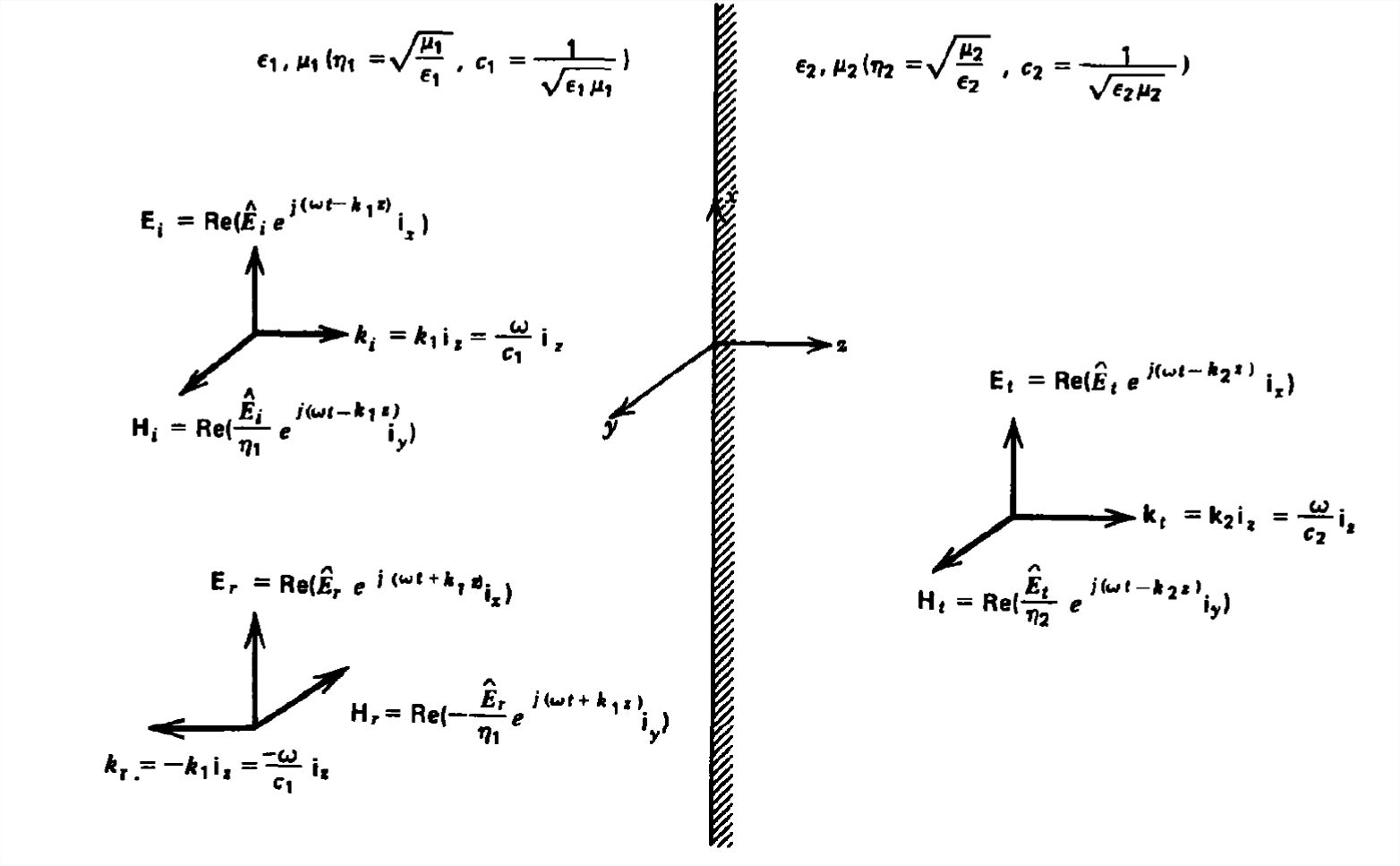
We replace the perfect conductor with a lossless dielectric of permittivity \(\varepsilon _{2}\) and permeability \(\mu _{2}\), as in Figure 7-14, with a uniform plane wave normally incident from a medium with permittivity \(\varepsilon _{1}\) and permeability \(\mu _{1}\). In addition to the incident and reflected fields for \(z <0\), there are transmitted fields which propagate in the \(+z\) direction within the medium for \(z >0\):

\[\]\[ \left.\begin{array}{ll}
\mathbf{E}_i(z, t)=\operatorname{Re}\left[\hat{E}_i e^{j\left(\omega t-k_1 z\right)} \mathbf{i}_x\right], & k_1=\omega \sqrt{\varepsilon_1 \mu_1} \\
\mathbf{H}_i(z, t)=\operatorname{Re}\left[\frac{\hat{E}_i}{\eta_1} e^{j\left(\omega t-k_1 z\right)} \mathbf{i}_y\right], & \eta_1=\sqrt{\frac{\mu_1}{\varepsilon_1}} \nonumber\\
\mathbf{E}_r(z, t)=\operatorname{Re}\left[\hat{E}_r e^{j\left(\omega t+k_1 z\right)} \mathbf{i}_x\right] & \nonumber\\
\mathbf{H}_r(z, t)=\operatorname{Re}\left[-\frac{\hat{E}_r}{\eta_1} e^{j\left(\omega t+k_1 z\right)} \mathbf{i}_y\right] &
\nonumber\end{array}\right\} \quad z<0 \]

\[ \left.\begin{array}{rlrl}
\mathbf{E}_t(z, t) & =\operatorname{Re}\left[\hat{E}_t e^{j\left(\omega t-k_2 z\right)} \mathbf{i}_x\right], & k_2=\omega \sqrt{\varepsilon_2 \mu_2} \nonumber \\
\mathbf{H}_t(z, t) & =\operatorname{Re}\left[\frac{\hat{E}_t}{\eta_2} e^{j\left(\omega t-k_2 z\right)} \mathbf{i}_y\right], & \eta_2=\sqrt{\frac{\mu_2}{\varepsilon_2}}
\nonumber \end{array}\right\} \quad z>0\]

It is necessary in (1) to use the appropriate wavenumber and impedance within each region. There is no wave traveling in the \(-z\) direction in the second region as we assume no boundaries or sources for \(z >0\).

Figure 7-14 A uniform plane wave normally incident upon a dielectric interface separating two different materials has part of its power reflected and part transmitted.

The unknown quantities \(\hat{E}_{r}\) and \(\hat{E}_{i}\), can be found from the boundary conditions of continuity of tangential \(\textbf{E}\) and \(\textbf{H}\) at \(z = 0\),

\[ \hat{E}_{i}+\hat{E}_{r}=\hat{E}_{t}\\
\frac{\hat{E}_{i}-\hat{E}_{r}}{\eta _{1}}=\frac{\hat{E}_{r}}{\eta _{2}} \]

from which we find the reflection \(R\) and transmission \(T\) field coefficients as

\[ R=\frac{\hat{E}_{r}}{\hat{E}_{i}}=\frac{\eta_{2}-\eta_{1}}{\eta_{2}+\eta_{1}}\\
T=\frac{\hat{E}_{t}}{\hat{E}_{i}}=\frac{2\eta_{2}}{\eta_{2}+\eta_{1}} \]

where from (2)

\[ 1+R=T \]

If both mediums have the same wave impedance, \(\eta_{1}=\eta_{2}\), there is no reflected wave.

Time-Average Power Flow

The time-average power flow in the region \(z <0\) is \(\)

\[ \begin{align} <S_{xi}>&=\frac{1}{2}\textrm{Re}\left [ \hat{E}_{x}\left ( z \right )\hat{H}_{y}^{\ast }\left ( z \right ) \right ] \\ &=\frac{1}{2\eta _{1}}\textrm{Re}\left [ \hat{E}_{i}e^{-jk_{1}z}+\hat{E}_{r}e^{+jk_{1}z} \right ]\left [ \hat{E}_{i}^{\ast }e^{+jk_{1}z}+\hat{E}_{r}^{\ast }e^{-jk_{1}z} \right ] \nonumber \\ &=
\frac{1}{2\eta _{1}}\left [ \left | \hat{E}_{i} \right |^{2} -\left | \hat{E}_{r} \right |^{2}\right ] \nonumber \\ {} & \quad +\frac{1}{2\eta _{1}}\underbrace{\textrm{Re}\left [ \hat{E}_{r}\hat{E}_{i}^{\ast }e^{+2jk_{1}z}-\hat{E}_{r}^{\ast }\hat{E}_{i}e^{-2jk_{1}z} \right ]}_0 \nonumber \end{align}  \]

The last term on the right-hand side of (5) is zero as it is the difference between a number and its complex conjugate, which is pure imaginary and equals \(2j\) times its imaginary part. Being pure imaginary, its real part is zero. Thus the time-average power flow just equals the difference in the power flows in the incident and reflected waves as found more generally in Section 7-3-2. The coupling terms between oppositely traveling waves have no time-average yielding the simple superposition of time-average powers:

\[ \begin{align} <S_{xi}>&=\frac{1}{2\eta _{1}}\left [ \left | \hat{E}_{i} \right |^{2} -\left | \hat{E}_{r} \right |^{2}\right ] \\ &=\frac{\left | \hat{E}_{i} \right |^{2}}{2\eta _{1}}\left [ 1-R^{2} \right ] \nonumber \end{align} \]

This net time-average power flows into the dielectric medium, as it also equals the transmitted power;

\[ <S_{xi}>=\frac{1}{2\eta _{2}}\left | \hat{E}_{t} \right |^{2}
=\frac{\left | \hat{E}_{i} \right |^{2}T^{2}}{2\eta _{2}}
=\frac{\left | \hat{E}_{i} \right |^{2}}{2\eta _{1}}\left [ 1-R^{2} \right ] \]

Lossy Dielectric

If medium \(2\) is lossy with Ohmic conductivity \(\sigma \), the solutions of (3) are still correct if we replace the permittivity \(\varepsilon_{2}\) by the complex permittivity \(\hat{\varepsilon}_{2}\),

\[ \hat{\varepsilon}_{2}= \varepsilon_{2}\left ( 1+\frac{\sigma }{j\omega \varepsilon_{2}} \right ) \]

so that the wave impedance in region \(2\) is complex:

\[ \eta _{2}= \sqrt{\mu _{2}/\hat{\varepsilon}_{2}} \]

We can easily explore the effect of losses in the low and large loss limits.

(a) Low Losses

If the Ohmic conductivity is small, we can neglect it in all terms except in the wavenumber \(k_2\):

\[ \lim_{\sigma /\omega \varepsilon _{2}\ll 1}k_{2}\approx \omega \sqrt{\varepsilon _{2}\mu _{2}}-\frac{j}{2}\sigma \sqrt{\frac{\mu _{2}}{\varepsilon _{2}}} \]

The imaginary part of \(k_2\) gives rise to a small rate of exponential decay in medium \(2\) as the wave propagates away from the \(z =0\) boundary.

(b) Large Losses

For large conductivities so that the displacement current is negligible in medium \(2\), the wavenumber and impedance in region \(2\) are complex:

\[ \lim_{\sigma /\omega \varepsilon _{2}\gg  1}\left\{\begin{matrix}
k_{2}= \frac{1-j}{\delta },\quad \delta =\sqrt{\frac{2}{\omega \mu _{2}\sigma }}\\ 
\eta _{2}=\sqrt{\frac{j\omega \mu _{2}}{\sigma }}=\frac{1+j}{\sigma \delta }
\end{matrix}\right.
\]

The fields decay within a characteristic distance equal to the skin depth \(\delta \). This is why communications to submerged submarines are difficult. For seawater, \(\mu _{2}=\mu _{0}=4\pi \times 10^{-7} \,\textrm{henry/m}\) and \(\sigma \approx 4 \,\textrm{siemens/m}\) so that for \(1 \,\textrm{MHz}\) signals, \(\delta \approx 0.25 \,\textrm{m}\). However, at \(100\,\textrm{Hz}\) the skin depth increases to \(25\,\textrm{meters}\). If a submarine is within this distance from the surface, it can receive the signals. However, it is difficult to transmit these low frequencies because of the large free space wavelength, \(\lambda \approx 3\times 10^{6}\,\textrm{m}\). Note that as the conductivity approaches infinity,

\[ \lim_{\sigma \rightarrow \infty }\left\{\begin{matrix}
k_{2}=\infty \\ 
\eta _{2}=0
\end{matrix}\right.\Rightarrow \left\{\begin{matrix}
R=-1\\ 
T=0
\end{matrix}\right. \]

so that the field solution approaches that of normal incidence upon a perfect conductor found in Section 7-5.

Example \(\PageIndex{1}\) EXAMPLE 7-1 DIELECTRIC COATING

A thin lossless dielectric with permittivity \(\varepsilon \) and permeability \(\mu \) is coated onto the interface between two infinite half-spaces of lossless media with respective properties \(\left ( \varepsilon_{1},\mu_{1} \right )\) and \(\left ( \varepsilon _{2},\mu _{2} \right )\), as shown in Figure 7-15. What coating parameters \(\varepsilon \) and \(\mu \)M and thickness \(d\) will allow all the time-average power

Figure 7-15 A suitable dielectric coating applied on the interface of discontinuity between differing media can eliminate reflections at a given frequency.

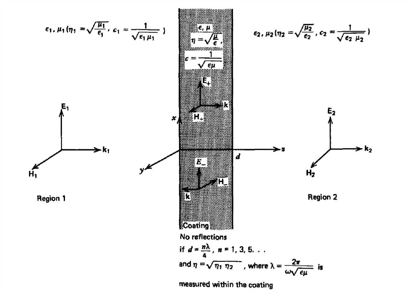
from region \(1\) to be transmitted through the coating to region \(2\)? Such coatings are applied to optical components such as lenses to minimize unwanted reflections and to maximize the transmitted light intensity.

SOLUTION

For all the incident power to be transmitted into region \(2\), there can be no reflected field in region \(1\), although we do have oppositely traveling waves in the coating due to the reflection at the second interface. Region \(2\) only has positively \(z\)-directed power flow. The fields in each region are thus of the following form:

Region 1

\[ \textbf{E}_{1}=\textrm{Re}\left [ \hat{E}_{1}e^{j\left ( \omega t-k_1 z \right )}\textbf{i}_{x} \right ],\quad k_1=\omega /c_{1}=\omega \sqrt{\varepsilon _{1}\mu _{1}} \nonumber \\
\textbf{H}_{1}=\textrm{Re}\left [ \frac{\hat{E}_{1}}{\eta _{1}}e^{j\left ( \omega t-k_1 z \right )}\textbf{i}_{y} \right ],\quad \eta_1=\sqrt{\frac{\mu _{1}}{\varepsilon _{1}}}  \nonumber \]

Coating

\[\begin{align}  \textbf{E}_{+}& =\textrm{Re}\left [ \hat{E}_{+}e^{j\left ( \omega t-kz \right )}\textbf{i}_{x} \right ],\quad k=\omega /c=\omega \sqrt{\varepsilon\mu} \nonumber \\
\textbf{H}_{+}& =\textrm{Re}\left [ \frac{\hat{E}_{+}}{\eta}e^{j\left ( \omega t-kz \right )}\textbf{i}_{y} \right ],\quad \eta_1=\sqrt{\frac{\mu}{\varepsilon}} \nonumber \\
\textbf{E}_{-}& =\textrm{Re}\left [ \hat{E}_{-}e^{j\left ( \omega t+kz \right )}\textbf{i}_{x} \right ] \nonumber \\
\textbf{H}_{-}& =\textrm{Re}\left [ -\frac{\hat{E}_{-}}{\eta}e^{j\left ( \omega t+kz \right )}\textbf{i}_{y} \right ]   \nonumber \end{align} \]

Region 2

\[  \textbf{E}_{2}=\textrm{Re}\left [ \hat{E}_{2}e^{j\left ( \omega t-k_2 z \right )}\textbf{i}_{x} \right ],\quad k_2=\omega /c_{2}=\omega \sqrt{\varepsilon _{2}\mu _{2}} \nonumber \\
\textbf{H}_{2}=\textrm{Re}\left [ \frac{\hat{E}_{2}}{\eta _{2}}e^{j\left ( \omega t-k_2 z \right )}\textbf{i}_{y} \right ],\quad \eta_2=\sqrt{\frac{\mu _{2}}{\varepsilon _{2}}}  \nonumber \]

Continuity of tangential \(\textbf{E}\) and \(\textbf{H}\) at \(z =0\) and \(z =d\) requires

\[ \hat{E}_{1}=\hat{E}_{+}+\hat{E}_{-},\quad  \frac{\hat{E}_{1}}{\eta _{1}}=\frac{\hat{E}_{+}-\hat{E}_{-}}{\eta } \nonumber \\
\hat{E}_{+}e^{-jkd}+\hat{E}_{-}e^{+jkd}=\hat{E}_{2}e^{-jk_{2}d} \nonumber \\
\frac{\hat{E}_{+}e^{-jkd}-\hat{E}_{-}e^{+jkd}}{\eta }=\frac{\hat{E}_{2}e^{-jk_{2}d}}{\eta _{2}} \nonumber \]

Each of these amplitudes in terms of \(\hat{E}_{1}\) is then

\[\begin{align} \hat{E}_{+}& =\frac{1}{2}\left ( 1+\frac{\eta }{\eta _{1}}\hat{E}_{1} \right ) \nonumber \\
\hat{E}_{-}& =\frac{1}{2}\left ( 1-\frac{\eta }{\eta _{1}}\hat{E}_{1} \right ) \nonumber \\
\hat{E}_{2}&=e^{jk_{2}d}\left [ \hat{E}_{+}e^{-jkd}+\hat{E}_{-}e^{+jkd} \right ] \\ &=\frac{\eta _{2}}{\eta }e^{jk_{2}d}\left [ \hat{E}_{+}e^{-jkd}-\hat{E}_{-}e^{+jkd} \right ] \nonumber \end{align} \]

Solving this last relation self-consistently required that 

\[ \hat{E}_{+}e^{-jkd}\left ( 1-\frac{\eta _{2}}{\eta}\right )+ \hat{E}_{-}e^{jkd}\left ( 1+\frac{\eta _{2}}{\eta}\right )=0 \]

Writing \(\hat{E}_{+}\) and \(\hat{E}_{-}\) in terms of \(\hat{E}_{1}\) yields

\[ \left ( 1+\frac{\eta}{\eta_{1}}\right )\left ( 1-\frac{\eta _{2}}{\eta}\right )+e^{2jkd}\left ( 1+\frac{\eta _{2}}{\eta}\right )\left ( 1-\frac{\eta}{\eta_{1}}\right )=0 \]

Since this relation is complex, the real and imaginary parts must separately be satisfied. For the imaginary part to be zero requires that the coating thickness \(d\) be an integral number of quarter wavelengths as measured within the coating,

\[ 2kd=n\pi \Rightarrow d=n\lambda /4,\quad n=1,2,3 \]

The real part then requires

\[ \left ( 1+\frac{\eta}{\eta_{1}}\right )\left ( 1-\frac{\eta _{2}}{\eta}\right )\pm \left ( 1+\frac{\eta _{2}}{\eta}\right )\left ( 1-\frac{\eta}{\eta_{1}}\right )=0\left\{\begin{matrix}
n\,\textrm{even}\\ n\,\textrm{odd} \end{matrix}\right. \]

For the upper sign where \(d\) is a multiple of half-wavelengths the only solution is

\[ \eta_{2}=\eta_{1}\quad \left ( d=n\lambda /4,\quad n=2,4,6,... \right ) \]

which requires that media \(1\) and \(2\) be the same so that the coating serves no purpose. If regions \(1\) and \(2\) have differing wave impedances, we must use the lower sign where \(d\) is an odd integer number of quarter wavelengths so that

\[ \eta ^{2}=\eta_{1}\eta_{2}\Rightarrow \eta = \sqrt{\eta_{1}\eta_{2}}\quad \left ( d=n\lambda /4,\quad n=1,3,5,... \right ) \]

Thus, if the coating is a quarter wavelength thick as measured within the coating, or any odd integer multiple of this thickness with its wave impedance equal to the geometrical average of the impedances in each adjacent region, all the time-average power flow in region \(1\) passes through the coating into region \(2\):

\[ \begin{align} <S_z> &=\frac{1}{2}\frac{\left | \hat{E}_{1} \right |^{2}}{\eta _{1}}=\frac{1}{2}\frac{\left | \hat{E}_{2} \right |^{2}}{\eta _{2}} \nonumber \\ &
=\frac{1}{2}\textrm{Re}\left [ \left ( \hat{E}_{+}e^{-jkd}+\hat{E}_{-}e^{+jkd} \right )\frac{\left ( \hat{E}_{+}^{\ast }e^{+jkd}-\hat{E}_{-}^{\ast }e^{-jkd} \right )}{\eta } \right ] \nonumber \\ &
=\frac{1}{2\eta }\left ( \left | \hat{E}_{+} \right |^{2}-\left | \hat{E}_{-} \right |^{2} \right ) \nonumber \end{align} \]

Note that for a given coating thickness \(d\), there is no reflection only at select frequencies corresponding to wavelengths \(d=n\lambda /4,\quad n=1,3,5,....\) For a narrow band of wavelengths about these select wavelengths, reflections are small. The magnetic permeability of coatings and of the glass used in optical components are usually that of free space while the permittivities differ. The permittivity of the coating \(\varepsilon\) is then picked so that

\[ \varepsilon = \sqrt{\varepsilon _{2}\varepsilon _{0}} \]

and with a thickness corresponding to the central range of the wavelengths of interest (often in the visible).