7.7: Uniform and Nonuniform Plane Waves

Our analysis thus far has been limited to waves propagating in the \(z\) direction normally incident upon plane interfaces. Although our examples had the electric field polarized in the \(x\) direction., the solution procedure is the same for the \(y\)-directed electric field polarization as both polarizations are parallel to the interfaces of discontinuity.

Propagation at an Arbitrary Angle

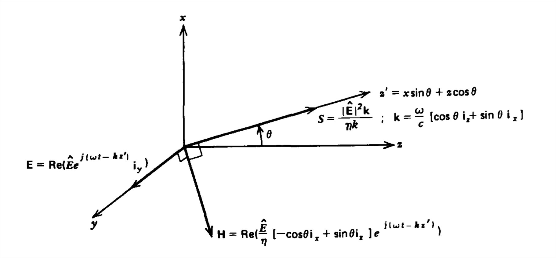
We now consider a uniform plane wave with power flow at an angle \(\theta \) to the \(z\) axis, as shown in Figure 7-16. The electric field is assumed to be \(y\) directed, but the magnetic field that is perpendicular to both \(\textbf{E}\) and \(\textbf{S}\) now has components in the \(x\) and \(z\) directions.

The direction of the power flow, which we can call \(z'\), is related to the Cartesian coordinates as

\[ z'=x\sin \theta +z\cos \theta  \]

so that the phase factor \(kz' \) can be written as

\[ \begin{align}kz'=k_{x}x+k_{z}z,\quad k_{x}& =k\sin \theta \\
k_{z}&=k\cos \theta \nonumber \end{align} \]

where the wavenumber magnitude is

\[ k=\omega \sqrt{\varepsilon \mu } \]

Figure 7-16 The spatial dependence of a uniform plane wave at an arbitrary angle \(\theta \) can be expressed in terms of a vector wavenumber \(\textbf{k}\) as \(e^{-j\textbf{k}\cdot r}\), where \(\textbf{k}\) is in the direction of power flow and has magnitude \(\omega /c\).

This allows us to write the fields as

\[ \begin{align}\textbf{E}& =\textbf{Re}\left [ \hat{E}e^{j\left ( \omega t-k_{z}x-k_{z}z \right )\textbf{i}_{y}} \right ] \\
\textbf{H}& =\textbf{Re}\left [ \frac{\hat{E}}{\eta }\left ( -\cos \theta \textbf{i}_{x}+\sin \theta \textbf{i}_{z} \right )e^{j\left ( \omega t-k_{z}x-k_{z}z \right )} \right ] \nonumber \end{align} \]

We note that the spatial dependence of the fields can be written as \(e^{-j\textbf{k}\cdot r}\), where the wavenumber is treated as a vector:

\[ \textbf{k}=k_x \textbf{i}_x+k_y \textbf{i}_y+k_z \textbf{i}_z \]

with

\[ \textbf{r}=x\textbf{i}_x+y\textbf{i}_y+z\textbf{i}_z \]

so that

\[ \textbf{k}\cdot \textbf{r}=k_x x+k_y y+k_z z \]

The magnitude of \(\textbf{k}\) is as given in (3) and its direction is the same as the power flow \(\textbf{S}\):

\[ \begin{align}\textbf{S}&=\textbf{E}\times \textbf{H}=\frac{\left | \hat{E} \right |^{2}}{\eta }\left ( \cos \theta \textbf{i}_{z}+\sin \theta \textbf{i}_{x} \right )\cos ^{2}\left ( \omega t-\textbf{k}\cdot \textbf{r} \right ) \\ &
=\frac{\left | \hat{E} \right |^{2}\textbf{k}}{ \omega \mu }\cos ^{2}\left ( \omega t-\textbf{k}\cdot \textbf{r} \right ) \nonumber \end{align} \]

where without loss of generality we picked the phase of \(\hat{E}\) to be zero so that it is real.

The Complex Propagation Constant

Let us generalize further by considering fields of the form

\[ \begin{align}
\textbf{E}&=\textrm{Re}\left [ \hat{\textbf{E}}e^{j\omega t}e^{-\boldsymbol{\gamma}\textbf{r}} \right ]= 
\textrm{Re}\left [ \hat{\textbf{E}}e^{j\left (\omega t-\textbf{k}\cdot \textbf{r} \right )}e^{-\boldsymbol{\alpha }\cdot \textbf{r}} \right ] \\
\textbf{H}& =\textrm{Re}\left [ \hat{\textbf{H}}e^{j\omega t}e^{-\boldsymbol{\gamma}\textbf{r}} \right ]= 
\textrm{Re}\left [ \hat{\textbf{H}}e^{j\left (\omega t-\textbf{k}\cdot \textbf{r} \right )}e^{-\boldsymbol{\alpha }\cdot \textbf{r}} \right ]
\nonumber \end{align} \]

where \(\boldsymbol{\gamma}\) is the complex propagation vector and \(\textbf{r}\) is the position vector of (6):

\[ \begin{align}\boldsymbol{\gamma}&=\boldsymbol{\alpha}+j\textbf{k}=\gamma_{x}\textbf{i}_{x}+\gamma_{y}\textbf{i}_{y}+\gamma_{z}\textbf{i}_{z} \\
\boldsymbol{\gamma}\cdot \textbf{r}&=\gamma_{x}x+\gamma_{y}y+\gamma_{z}z \nonumber \end{align} \]

We have previously considered uniform plane waves in lossless media where the wavenumber \(\textbf{k}\) is pure real and \(z\) directed with \(\alpha=0\) so that \(\boldsymbol{\gamma}\) is pure imaginary. The parameter \(\boldsymbol{\alpha }\) represents the decay rate of the fields even though the medium is lossless. If \(\boldsymbol{\alpha }\) is nonzero, the solutions are called nonuniform plane waves. We saw this decay in our quasi-static solutions of Laplace's equation where solutions had oscillations in one direction but decay in the perpendicular direction. We would expect this evanescence to remain at low frequencies.

The value of the assumed form of solutions in (9) is that the \(\textrm{del}\left ( \boldsymbol{\nabla}\right )\) operator in Maxwell's equations can be replaced by the vector operator \(-\boldsymbol{\gamma}\):

\[ \begin{align}\boldsymbol{\nabla}&= \frac{\partial }{\partial x}\textbf{i}_{x}+\frac{\partial }{\partial y}\textbf{i}_{y}+\frac{\partial }{\partial z}\textbf{i}_{z} \\&
=-\gamma_{x}\textbf{i}_{x}-\gamma_{y}\textbf{i}_{y}-\gamma_{z}\textbf{i}_{z} \nonumber \\&
=-\boldsymbol{\gamma } \nonumber \end{align} \]

This is true because any spatial derivatives only operate on the exponential term in (9). Then the source free Maxwell's equations can be written in terms of the complex amplitudes as

\[ -\boldsymbol{\gamma }\times \hat{\textbf{E}}= -j\omega \mu \hat{\textbf{H}}\\
-\boldsymbol{\gamma }\times \hat{\textbf{H}}= j\omega \varepsilon  \hat{\textbf{E}}  \\
-\boldsymbol{\gamma }\cdot  \varepsilon \hat{\textbf{E}}= 0 \\
-\boldsymbol{\gamma }\cdot  \hat{\textbf{H}}= 0  \]

The last two relations tell us that \(\boldsymbol{\gamma }\) is perpendicular to both \(\textbf{E}\) and \(\textbf{H}\). If we take \(\boldsymbol{\gamma }\times \) the top equation and use the second equation, we have

\[ \begin{align}-\boldsymbol{\gamma }\times \left ( \boldsymbol{\gamma }\times \hat{\textbf{E}} \right )&=-j\omega \mu \left ( \boldsymbol{\gamma }\times \hat{\textbf{H}} \right )=-j\omega \mu \left ( -j\omega \varepsilon \hat{\textbf{E}} \right ) \\ &=-\omega^{2}\mu \varepsilon \hat{\textbf{E}} \nonumber \end{align} \]

The double cross product can be expanded as

\[ \begin{align}-\boldsymbol{\gamma }\times \left ( \boldsymbol{\gamma }\times \hat{\textbf{E}} \right )&=-\boldsymbol{\gamma } \left ( \boldsymbol{\gamma }\cdot  \hat{\textbf{E}} \right )+\left ( \boldsymbol{\gamma }\cdot \boldsymbol{\gamma } \right )\hat{\textbf{E}} \\ &=\left ( \boldsymbol{\gamma }\cdot \boldsymbol{\gamma } \right )\hat{\textbf{E}}=-\omega^{2}\mu \varepsilon \hat{\textbf{E}} \nonumber \end{align} \]

The \(\boldsymbol{\gamma }\cdot \hat{\textbf{E}}\) term is zero from the third relation in (12). The dispersion relation is then

\[ \boldsymbol{\gamma }\cdot \boldsymbol{\gamma } =\left ( \alpha ^{2}-k^{2}+2j\boldsymbol{\alpha} \cdot \textbf{k} \right )=-\omega ^{2}\mu \varepsilon  \]

For solution, the real and imaginary parts of (15) must be separately equal:

\[ \alpha ^{2}-k^{2}=-\omega ^{2}\mu \varepsilon \\
\boldsymbol{\alpha} \cdot \textbf{k}=0 \]

When \(\boldsymbol{\alpha}=0\), (16) reduces to the familiar frequency-wavenumber relation of Section 7-3-4.

The last relation now tells us that evanescence (decay) in space as represented by \(\boldsymbol{\alpha}\) is allowed by Maxwell's equations, but must be perpendicular to propagation represented by \(\textbf{k}\).

We can compute the time-average power flow for fields of the form of (9) using (12) in terms of either \(\hat{\textbf{E}}\) or \(\hat{\textbf{H}}\) as follows:

\[ \begin{align}<\textbf{S}>&=\frac{1}{2}\textrm{Re}\left ( \hat{\textbf{E}}\times \hat{\textbf{H}}^{\ast } \right ) \\ &
=-\frac{1}{2}\textrm{Re}\left ( \hat{\textbf{E}}\times \frac{\boldsymbol{\gamma }^{\ast }\times \hat{\textbf{E}}^{\ast }}{j\omega \mu } \right ) \nonumber \\ &
=-\frac{1}{2}\textrm{Re}\left (\frac{\boldsymbol{\gamma }^{\ast }\left | \hat{\textbf{E}}\right |^{2}- \hat{\textbf{E}}^{\ast }\left (\boldsymbol{\gamma }^{\ast }\cdot \hat{\textbf{E}}\right )}{j\omega \mu } \right ) \nonumber \\ &
=\frac{1}{2}\frac{\textbf{k}}{\omega \mu }\left | \hat{\textbf{E}}\right |^{2}+\frac{1}{2}\textrm{Re}\left ( \frac{ \hat{\textbf{E}}^{\ast }\left (\boldsymbol{\gamma }^{\ast }\cdot \hat{\textbf{E}}\right )}{j\omega \mu } \right ) \nonumber \\ 
<\textbf{S}>&=\frac{1}{2}\textrm{Re}\left ( \hat{\textbf{E}}\times \hat{\textbf{H}}^{\ast } \right ) \nonumber \\ &
=-\frac{1}{2}\textrm{Re}\left ( \frac{\left ( \boldsymbol{\gamma }\times \hat{\textbf{H}} \right )}{j\omega \varepsilon  }\times \hat{\textbf{H}}^{\ast } \right ) \nonumber \\ &
=\frac{1}{2}\textrm{Re}\left (\frac{\boldsymbol{\gamma }\left | \hat{\textbf{H}}\right |^{2}- \hat{\textbf{H}}^{\ast }\left (\boldsymbol{\gamma }\cdot \hat{\textbf{H}}^{\ast }\right )}{j\omega \varepsilon  } \right ) \nonumber \\ & 
=\frac{1}{2}\frac{\textbf{k}}{\omega\varepsilon }\left | \hat{\textbf{H}}\right |^{2}-\frac{1}{2}\textrm{Re}\left ( \frac{ \hat{\textbf{H}}\left (\boldsymbol{\gamma }\cdot \hat{\textbf{H}}^{\ast }\right )}{j\omega \varepsilon } \right ) 
\nonumber \end{align} \]

Although both final expressions in (17) are equivalent, it is convenient to write the power flow in terms of either \(\hat{\textbf{E}}\) or \(\hat{\textbf{H}}\). When \(\hat{\textbf{E}}\) is perpendicular to both the real vectors \(\boldsymbol{\alpha }\) and \(\boldsymbol{\beta }\), defined in (10) and (16), the dot product \(\boldsymbol{\gamma }^{\ast }\cdot \hat{\textbf{E}}\) is zero. Such a mode is called transverse electric (TE), and we see in (17) that the time-average power flow is still in the direction of the wavenumber \(\textbf{k}\). Similarly, when \(\textbf{H}\) is perpendicular to \(\boldsymbol{\alpha }\) and \(\boldsymbol{\beta }\), the dot product \(\boldsymbol{\gamma }\cdot \hat{\textbf{H}}^{\ast }\) is zero and we have a transverse magnetic (TM) mode. Again, the time-average power flow in (17) is in the direction of \(\textbf{k}\). The magnitude of \(\textbf{k}\) is related to \(\omega\) in (16).

Note that our discussion has been limited to lossless systems. We can include Ohmic losses if we replace \(\varepsilon\) by the complex permittivity \(\hat{\varepsilon }\) of Section 7-4-3 in (15) and (17). Then, there is always decay \((a\neq 0)\) because of Ohmic dissipation (see Problem 22).

Nonuniform Plane Waves

We can examine nonuniform plane wave solutions with nonzero \(\boldsymbol{\alpha }\) by considering a current sheet in the \(z =0\) plane, which is a traveling wave in the \(x\) direction:

\[ K_{x}\left ( z= 0 \right )= K_{0}\cos \left ( \omega t-k_{x}x \right )=\textrm{Re}\left ( K_{0}e^{j\left ( \omega t-k_{x}x \right )} \right ) \]

The \(x\)-directed surface current gives rise to a \(y\)-directed magnetic field. Because the system does not depend on the \(y\) coordinate, solutions are thus of the following form:

\[ H_{y}= \left\{\begin{matrix}
\textrm{Re}\left ( \hat{H}_{1}e^{j\omega t}e^{-\boldsymbol{\gamma }_{1}\cdot \textbf{r}} \right ),\quad z> 0\\ 
\textrm{Re}\left ( \hat{H}_{2}e^{j\omega t}e^{-\boldsymbol{\gamma }_{2}\cdot \textbf{r}} \right ),\quad z< 0
\end{matrix}\right.\\
\textbf{E}= \left\{\begin{matrix}
\textrm{Re}\left [ -\frac{\boldsymbol{\gamma }_{1}\times \hat{H}_{1}}{j\omega \varepsilon }\textbf{i}_{y}e^{j\omega t}e^{-\boldsymbol{\gamma }_{1}\cdot \textbf{r}} \right ],\quad z> 0\\ 
\textrm{Re}\left [ -\frac{\boldsymbol{\gamma }_{2}\times \hat{H}_{2}}{j\omega \varepsilon }\textbf{i}_{y}e^{j\omega t}e^{-\boldsymbol{\gamma }_{2}\cdot \textbf{r}} \right ],\quad z< 0
\end{matrix}\right. \]

where \(\boldsymbol{\gamma }_{1}\) and \(\boldsymbol{\gamma }_{2}\) are the complex propagation vectors on each side of the current sheet:

\[ \boldsymbol{\gamma }_{1}=\gamma _{1x}\textbf{i}_{x}+\gamma _{1z}\textbf{i}_{z}\\
\boldsymbol{\gamma }_{2}=\gamma _{2x}\textbf{i}_{x}+\gamma _{2z}\textbf{i}_{z} \]

The boundary condition of the discontinuity of tangential \(\textbf{H}\) at \(z =0\) equaling the surface current yields

\[ -\hat{H}_{1}e^{-\boldsymbol{\gamma }_{1x}x}+\hat{H}_{2}e^{-\boldsymbol{\gamma }_{2x}x}=K_{0}e^{-jk_{x}x} \]

which tells us that the \(x\) components of the complex propagation vectors equal the trigonometric spatial dependence of the surface current:

\[ \gamma_{1x}+\gamma_{2x}=jk_{x} \]

The \(z\) components of \(\boldsymbol{\gamma }_{1}\) and \(\boldsymbol{\gamma }_{2}\) are then determined from (15) as

\[ \gamma_{x}^{2}+\gamma_{z}^{2}=-\omega ^{2}\varepsilon \mu \Rightarrow \gamma _{z}=\pm \left ( k_{x}^{2}-\omega ^{2}\varepsilon \mu  \right )^{1/2} \]

If \(k_{x}^{2}<\omega ^{2}\varepsilon \mu\), \(\gamma _{z}\) is pure imaginary representing propagation and we have uniform plane waves. If \(k_{x}^{2}>\omega ^{2}\varepsilon \mu\), then \(\gamma _{z}\) is pure real representing evanescence in the \(z\) direction so that we generate nonuniform plane waves. When \(w =0\), (23) corresponds to Laplacian solutions that oscillate in the \(x\) direction but decay in the \(z\) direction.

The \(z\) component of \(\boldsymbol{\gamma }\) is of opposite sign in each region,

\[ \gamma _{1z}=-\gamma _{2z}=+\left ( k_{x}^{2}-\omega ^{2}\varepsilon \mu \right )^{1/2} \]

as the waves propagate or decay away from the sheet. Continuity of the tangential component of \(\textbf{E}\) requires

\[ \gamma _{1z}\hat{H}_{1}=-\gamma _{2z}\hat{H}_{2}\Rightarrow \hat{H}_{2}=-\hat{H}_{1}=K_{0}/2 \]

If \(k_{x}=0\), we re-obtain the solution of Section 7-4-1. Increasing \(k_{x}\). generates propagating waves with power flow in the \(k_{x}\textbf{i}_{x}\pm k_{z}\textbf{i}_{z}\) directions. At \(k_{x}^{2}=\omega ^{2}\varepsilon \mu ,\,k_{z}= 0\) so that the power flow is purely \(x\) directed with no spatial dependence on \(z\). Further increasing \(k_{x}\) converts \(k_{z}\) to \(\alpha _{z}\) as \(\gamma _{z}\) becomes real and the fields decay with \(z\).