
7.8: Oblique Incidence onto a Perfect Conductor
- Page ID
- 48163

E Field Parallel to the Interface
In Figure 7-17a we show a uniform plane wave incident upon a perfect conductor with power flow at an angle \(\theta _{i}\) to the normal. The electric field is parallel to the surface with the magnetic field having both \(x\) and \(z\) components:
\[ \textbf{E}_{i}= \textrm{Re}\left [ \hat{E}_{i}e^{j\left ( \omega t-k_{xi}x-k_{zi}z \right )}\textbf{i}_{y} \right ] \\
\textbf{H}_{i}= \textrm{Re}\left [ \frac{\hat{E}_{i}}{\eta }\left ( -\cos \theta _{i}\textbf{i}_{x}+\sin \theta _{i}\textbf{i}_{z} \right )e^{j\left ( \omega t-k_{xi}x-k_{zi}z \right )} \right ] \]
where
\[ \left.\begin{matrix}
k_{xi}=k\,\sin \theta_{i}\\
k_{zi}=k\,\cos \theta_{i}\end{matrix}\right\} \quad k= \omega \sqrt{\varepsilon \mu },\quad \eta = \sqrt{\frac{\mu}{\epsilon } } \]
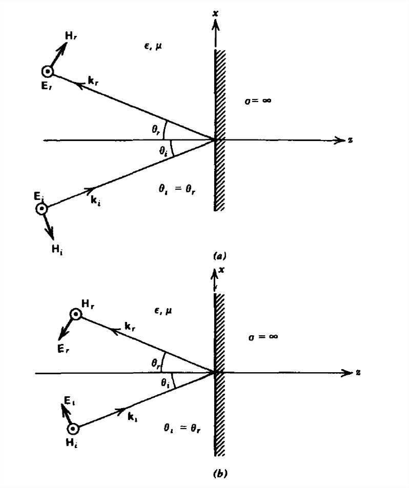
There are no transmitted fields within the perfect conductor, but there is a reflected field with power flow at angle \(\theta _{r}\) from the interface normal. The reflected electric field is also in the \(y\) direction so the magnetic field, which must be perpendicular to both \(\textbf{E}\) and \(\textbf{S}=\textbf{E}\times \textbf{H}\), is in the direction shown in Figure 7-17a:
\[\textbf{E}_{r}= \textrm{Re}\left [ \hat{E}_{r}e^{j\left ( \omega t-k_{xr}x+k_{zr}z \right )}\textbf{i}_{y} \right ] \\
\textbf{H}_{r}= \textrm{Re}\left [ \frac{\hat{E}_{r}}{\eta }\left ( \cos \theta _{r}\textbf{i}_{x}+\sin \theta _{r}\textbf{i}_{z} \right )e^{j\left ( \omega t-k_{xr}x+k_{zr}z \right )} \right ] \]
where the reflected wavenumbers are
\[ k_{xr}=k\,\sin \theta_{r}\\
k_{zr}=k\,\cos \theta_{r} \]
At this point we do not know the angle of reflection \(\theta_{r}\) or the reflected amplitude \(\hat{E}_{r}\). They will be determined from the boundary conditions at \(z =0\) of continuity of tangential \(\textbf{E}\) and normal \(\textbf{B}\). Because there are no fields within the perfect conductor these boundary conditions at \(z =0\) are
\[\begin{align} \hat{E}_{i}e^{-jk_{xi}x}+\hat{E}_{r}e^{-jk_{xr}x}& =0 \\
\frac{\mu }{\eta }\left ( \hat{E}_{i}\sin \theta _{i}e^{-jk_{xi}x}+\hat{E}_{r}\sin \theta _{r}e^{-jk_{xr}x} \right )&=0 \nonumber \end{align} \]
These conditions must be true for every value of \(x\) along \(z = 0\) so that the phase factors given in (2) and (4) must be equal,
\[ k_{xi}=k_{xr}\Rightarrow \theta _{i}=\theta _{r}\equiv \theta \]
giving the well-known rule that the angle of incidence equals the angle of reflection. The reflected field amplitude is then
\[ \hat{E}_{r}=-\hat{E}_{i} \]
with the boundary conditions in (5) being redundant as they both yield (7). The total fields are then:
\[ \begin{align}E_{y}&=\textrm{Re}\left [ \hat{E}_{i}\left ( e^{-jk_{z}z}-e^{+jk_{z}z} \right )e^{j\left ( \omega t-k_{z}x \right )} \right ] \\ &
=2E_{i}\sin k_{z}z\sin \left ( \omega t-k_{x}x \right ) \nonumber \\
\textbf{H} &=\textrm{Re}\left [ \frac{\hat{E}_{i}}{\eta }\left [ \cos \theta \left ( -e^{-jk_{z}z}-e^{+jk_{z}z} \right )\textbf{i}_{x}+\sin \theta \left ( e^{-jk_{z}z}-e^{+jk_{z}z} \right )\textbf{i}_{z} \right ]e^{j\left ( \omega t-k_{z}x \right )} \right ] \nonumber \\ &
= \frac{2E_{i}}{\eta }\left [ -\cos \theta \cos k_{z}z\cos \left ( \omega t-k_{x}x \right )\textbf{i}_{x} +\sin \theta \sin k_{z}z\sin \left ( \omega t-k_{x}x \right )\textbf{i}_{z}\right ] \nonumber \end{align} \]
where without loss of generality we take \(\hat{E}_{i}\) to be real.
We drop the \(i\) and \(r\) subscripts on the wavenumbers and angles because they are equal. The fields travel in the \(x\) direction parallel to the interface, but are stationary in the \(z\) direction. Note that another perfectly conducting plane can be placed at distances \(d\) to the left of the interface at
\[ k_{z}d=n\pi \]
where the electric field is already zero without disturbing the solutions of (8). The boundary conditions at the second conductor are automatically satisfied. Such a structure is called a waveguide and is discussed in Section 8-6.
Because the tangential component of \(\textbf{H}\) is discontinuous at \(z =0\), a traveling wave surface current flows along the interface,
\[ K_{y}=-H_{x}\left ( z=0 \right )=\frac{2E_{i}}{\eta }\cos \theta \cos \left ( \omega t-k_{x}x \right ) \]
From (8) we compute the time-average power flow as
\[ \begin{align}<\textbf{S}>&=\frac{1}{2}\textrm{Re}\left [ \hat{\textbf{E}}\left ( x,z \right )\times\hat{\textbf{H}}^{\ast }\left ( x,z \right ) \right ] \\ &
=\frac{2E_{i}^{2}}{\eta }\sin \theta \sin ^{2}k_{z}z\textbf{i}_{x} \nonumber \end{align} \]
We see that the only nonzero power flow is in the direction parallel to the interfacial boundary and it varies as a function of \(z\).
H Field Parallel to the Interface
If the \(\textbf{H}\) field is parallel to the conducting boundary, as in Figure 7-17b, the incident and reflected fields are as follows:
\[ \begin{align}\textbf{E}_{i}&= \textrm{Re}\left [ \hat{E}_{i}\left ( \cos \theta _{i}\textbf{i}_{x}-\sin \theta _{i}\textbf{i}_{z} \right )e^{j\left ( \omega t-k_{xi}x-k_{zi}z \right )}\right ] \\
\textbf{H}_{i}&= \textrm{Re}\left [ \frac{\hat{E}_{i}}{\eta }e^{j\left ( \omega t-k_{xi}x-k_{zi}z \right )} \textbf{i}_{y}\right ] \nonumber \\
\textbf{E}_{r}&= \textrm{Re}\left [ \hat{E}_{r}\left ( -\cos \theta _{r}\textbf{i}_{x}-\sin \theta _{r}\textbf{i}_{z} \right )e^{j\left ( \omega t-k_{xr}x+k_{zr}z \right )}\right ] \nonumber \\
\textbf{H}_{r}&= \textrm{Re}\left [ \frac{\hat{E}_{r}}{\eta }e^{j\left ( \omega t-k_{xr}x+k_{zr}z \right )} \textbf{i}_{y}\right ] \nonumber \end{align} \]
The tangential component of \(\textbf{E}\) is continuous and thus zero at \(z = 0\):
\[ \hat{E}_{i}\cos \theta _{i}e^{-jk_{xi}x}-\hat{E}_{r}\cos \theta _{r}e^{-jk_{xr}x}=0 \]
There is no normal component of \(\textbf{B}\). This boundary condition must be satisfied for all values of \(x\) so again the angle of incidence must equal the angle of reflection \(\left ( \theta _{i}=\theta _{r} \right )\) so that
\[ \hat{E}_{i}=\hat{E}_{r} \]
The total \(\textbf{E}\) and \(\textbf{H}\) fields can be obtained from (12) by adding the incident and reflected fields and taking the real part;
\[ \begin{align}\textbf{E} &=\textrm{Re}\left [ \hat{E}_{i}\left [ \cos \theta \left ( e^{-jk_{z}z}-e^{+jk_{z}z} \right )\textbf{i}_{x}-\sin \theta \left ( e^{-jk_{z}z}+e^{+jk_{z}z} \right )\textbf{i}_{z} \right ]e^{j\left ( \omega t-k_{z}x \right )} \right ] \\ &
=2E_{i}\left [ \cos \theta \sin k_{z}z\sin\left ( \omega t-k_{x}x \right )\textbf{i}_{x} -\sin \theta \cos k_{z}z\cos \left ( \omega t-k_{x}x \right )\textbf{i}_{z}\right ]
\nonumber \\
\textbf{H} &=\textrm{Re}\left [ \frac{\hat{E}_{i}}{\eta }\left ( e^{-jk_{z}z}+e^{+jk_{z}z} \right )e^{j\left ( \omega t-k_{z}x \right )}\textbf{i}_{y} \right ] \nonumber \\ &
=\frac{2E_{i}}{\eta }\cos k_{z}z\cos \left ( \omega t-k_{x}x \right )\textbf{i}_{y}
\nonumber \end{align} \]
The surface current on the conducting surface at \(z =0\) is given by the tangential component of \(\textbf{H}\)
\[ K_{y}\left ( z=0 \right )=H_{y}\left ( z=0 \right )=\frac{2E_{i}}{\eta }\cos \left ( \omega t-k_{x}x \right ) \]
while the surface charge at \(z = 0\) is proportional to the normal component of electric field,
\[ \sigma _{f}\left ( z=0 \right )=-\varepsilon E_{z}\left ( z=0 \right )=2\varepsilon E_{i}\sin \theta \cos \left ( \omega t-k_{x}x \right ) \]
Note that (16) and (17) satisfy conservation of current on the conducting surface,
\[ \nabla _{\Sigma }\cdot \textbf{K}+\frac{\partial \sigma _{f}}{\partial t}=0\Rightarrow \frac{\partial K_{x}}{\partial x}+\frac{\partial \sigma _{f}}{\partial t}=0 \]
where
\[ \nabla _{\Sigma }=\frac{\partial }{\partial x}\textbf{i}_{x}+\frac{\partial }{\partial y}\textbf{i}_{y} \nonumber \]
is the surface divergence operator. The time-average power flow for this polarization is also \(x\) directed:
\[ \begin{align}<\textbf{S}>&=\frac{1}{2}\textrm{Re}\left [ \hat{\textbf{E}}\times\hat{\textbf{H}}^{\ast }\right ] \\ &
=\frac{2E_{i}^{2}}{\eta }\sin \theta \cos ^{2}k_{z}z\textbf{i}_{x} \nonumber \end{align} \]