7.9: Oblique Incidence Onto a Dielectric

\(E\) Parallel to the Interface

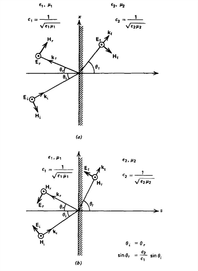
A plane wave incident upon a dielectric interface, as in Figure 7-18a, now has transmitted fields as well as reflected fields. For the electric field polarized parallel to the interface, the fields in each region can be expressed as

\[ \begin{align}\textbf{E}_{i}&= \textrm{Re}\left [ \hat{E}_{i}e^{j\left ( \omega t-k_{xi}x-k_{zi}z \right )}\textbf{i}_{y}\right ] \\
\textbf{H}_{i}&= \textrm{Re}\left [ \frac{\hat{E}_{i}}{\eta_{1} }\left ( -\cos \theta _{i}\textbf{i}_{x}+\sin \theta _{i}\textbf{i}_{z} \right )e^{j\left ( \omega t-k_{xi}x-k_{zi}z \right )}\right ] \nonumber \\
\textbf{E}_{r}&= \textrm{Re}\left [ \hat{E}_{r}e^{j\left ( \omega t-k_{xr}x+k_{zr}z \right )}\textbf{i}_{y}\right ] \nonumber \\
\textbf{H}_{r}&= \textrm{Re}\left [ \frac{\hat{E}_{r}}{\eta_{2} }\left ( \cos \theta _{r}\textbf{i}_{x}+\sin \theta _{r}\textbf{i}_{z} \right )e^{j\left ( \omega t-k_{xr}x+k_{zr}z \right )}\right ]
\nonumber \\
\textbf{E}_{t}&= \textrm{Re}\left [ \hat{E}_{t}e^{j\left ( \omega t-k_{xt}x-k_{zt}z \right )}\textbf{i}_{y}\right ] \nonumber \\
\textbf{H}_{t}&= \textrm{Re}\left [ \frac{\hat{E}_{t}}{\eta_{3} }\left ( -\cos \theta _{t}\textbf{i}_{x}+\sin \theta _{t}\textbf{i}_{z} \right )e^{j\left ( \omega t-k_{xt}x-k_{zt}z \right )}\right ] \nonumber \end{align} \]

where \(\theta _{i}\), \(\theta _{r}\), and \(\theta _{t}\) are the angles from the normal of the incident, reflected, and transmitted power flows. The wavenumbers in each region are

\[ k_{xi}=k_{1}\sin \theta _{i},\quad k_{xr}=k_{1}\sin \theta _{r},\quad k_{xt}=k_{2}\sin \theta _{t}\\
k_{zi}=k_{1}\sin \theta _{i},\quad k_{zr}=k_{1}\sin \theta _{r},\quad k_{zt}=k_{2}\sin \theta _{t} \]

where the wavenumber magnitudes, wave speeds, and wave impedances are

\[ k_{1}=\frac{\omega}{c_{1}},\quad k_{2}=\frac{\omega}{c_{2}},\quad c_{1}=\frac{1}{\sqrt{\varepsilon _{1}\mu _{1}}}\\
\eta _{1}=\sqrt{\frac{\mu _{1}}{\varepsilon _{1}}},\quad \eta _{2}=\sqrt{\frac{\mu _{2}}{\varepsilon _{2}}},\quad c_{2}=\frac{1}{\sqrt{\varepsilon _{2}\mu _{2}}} \]

The unknown angles and amplitudes in (1) are found from the boundary conditions of continuity of tangential \(\textbf{E}\) and \(\textbf{H}\) at the \( z =0\) interface.

\[ \hat{E}_{i}e^{-jk_{xi}x}+\hat{E}_{r}e^{-jk_{xr}x}=\hat{E}_{t}e^{-jk_{xt}x}\\
\frac{-\hat{E}_{i}\cos \theta _{i}e^{-jk_{xi}x}+\hat{E}_{r}\cos \theta _{r}e^{-jk_{xr}x}}{\eta _{1}}=-\frac{\hat{E}_{t}\cos \theta _{t}e^{-jk_{xt}x}}{\eta_{2}} \]

These boundary conditions must be satisfied point by point for all \(x\). This requires that the exponential factors also be

Figure 7-18 A uniform plane wave obliquely incident upon a dielectric interface also has its angle of incidence equal to the angle of reflection while the transmitted angle is given by Snell's law. (a) Electric field polarized parallel to the interface. (b) Magnetic field parallel to the interface.

equal so that the \(x\) components of all wavenumbers must be equal,

\[ k_{xi}=k_{xr}=k_{xt}\Rightarrow k_{1}\sin \theta _{i}=k_{1}\sin \theta _{r}=k_{2}\sin \theta _{t} \]

which relates the angles as

\[ \theta _{r}=\theta _{i}\]
\[\sin \theta _{t}=\left ( c_{2}/c_{1} \right )\sin \theta _{i} \]

As before, the angle of incidence equals the angle of reflection. The transmission angle obeys a more complicated relation called Snell's law relating the sines of the angles. The angle from the normal is largest in that region which has the faster speed of electromagnetic waves.

In optics, the ratio of the speed of light in vacuum, \(c_{0}=1/\sqrt{\varepsilon_{0} \mu _{0}}\), to the speed of light in the medium is defined as the index of refraction,

\[ n_1=c_{0}/c_{1},\quad n_2=c_{0}/c_{2} \]

which is never less than unity. Then Snell's law is written as

\[ \sin \theta _{t}=\left ( n_{1}/n_{2} \right )\sin \theta _{i} \]

With the angles related as in (6), the reflected and transmitted field amplitudes can be expressed in the same way as for normal incidence (see Section 7-6-1) if we replace the wave impedances by \(\eta \rightarrow \eta /\cos \theta \) to yield

\[ R=\frac{\hat{E}_{r}}{\hat{E}_{i}}=\frac{\frac{\eta _{2}}{\cos \theta _{t}}-\frac{\eta _{1}}{\cos \theta _{i}}}{\frac{\eta _{2}}{\cos \theta _{t}}+\frac{\eta _{1}}{\cos \theta _{i}}}=\frac{\eta _{2}\cos \theta _{i}-\eta _{1}\cos \theta _{t}}{\eta _{2}\cos \theta _{i}+\eta _{1}\cos \theta _{t}}\\
T=\frac{\hat{E}_{t}}{\hat{E}_{i}}=\frac{2\eta _{2}}{\cos\theta _{t}\left ( \frac{\eta _{2}}{\cos \theta _{t}}+\frac{\eta _{1}}{\cos \theta _{i}} \right )}=\frac{2\eta _{2}\cos\theta _{i} }{\eta _{2}\cos \theta _{i}+\eta _{1}\cos \theta _{t}} \]

In (4) we did not consider the boundary condition of continuity of normal \(\textbf{B}\) at \(z =0\). This boundary condition is redundant as it is the same condition as the upper equation in (4):

\[ \frac{\mu _{1}}{\eta _{1}}\left ( \hat{E}_{i}+\hat{E}_{r} \right )\sin \theta _{i}=\frac{\mu _{2}}{\eta _{2}} \hat{E}_{t}\sin \theta _{t}\Rightarrow \left ( \hat{E}_{i}+\hat{E}_{r} \right )=\hat{E}_{t} \]

where we use the relation between angles in (6). Since

\[ \frac{\mu _{1}}{\eta _{1}}=\sqrt{\mu_{1} \varepsilon_{1}}=\frac{1}{c_{1}},\quad \frac{\mu _{2}}{\eta _{2}}=\sqrt{\mu_{2} \varepsilon_{2}}=\frac{1}{c_{2}} \]

the trigonometric terms in (11) cancel due to Snell's law. There is no normal component of \(\textbf{D}\) so it is automatically continuous across the interface.

Brewster's Angle of No Reflection

We see from (10) that at a certain angle of incidence, there is no reflected field as \(R=0\). This angle is called Brewster's angle:

\[ R=0\Rightarrow \eta _{2}\cos \theta _{i}=\eta _{1}\cos \theta _{t} \]

By squaring (13), replacing the cosine terms with sine terms \(\left ( \cos ^{2}\theta =1-\sin ^{2}\theta  \right )\), and using Snell's law of (6), the Brewster angle \(\theta _{B}\) is found as

\[ \sin ^{2}\theta_{B}=\frac{1-\varepsilon _{2}\mu _{1}/\left ( \varepsilon _{1}\mu _{2} \right )}{1-\left ( \mu _{1}/\mu _{2} \right )^{2}} \]

There is not always a real solution to (14) as it depends on the material constants. The common dielectric case, where \(\mu_{1}=\mu_{2}\equiv \mu \) but \(\varepsilon_{1}\neq \varepsilon_{2}\), does not have a solution as the right-hand side of (14) becomes infinite. Real solutions to (14) require the right-hand side to be between zero and one. A Brewster's angle does exist for the uncommon situation where \(\varepsilon_{1}= \varepsilon_{2}\) and \(\mu_{1}\neq \mu_{2}\):

\[ \sin ^{2}\theta _{B}=\frac{1}{1+\mu_{1}/\mu_{2}}\Rightarrow \tan \theta _{B}=\sqrt{\frac{\mu_{2}}{\mu_{1}}} \]

At this Brewster's angle, the reflected and transmitted power flows are at right angles \(\left ( \theta _{B}+\theta _{t}=\pi /2 \right )\) as can be seen by using (6), (13), and (14):

\[ \begin{align}\cos \left ( \theta _{B}+\theta _{t}\right )&=\cos\theta _{B}\cos\theta _{t}-\sin \theta _{B}\sin \theta _{t} \\ &
=\cos^{2}\theta _{B}\sqrt{\frac{\mu _{2}}{\mu _{1}}}-\sin^{2}\theta _{B}\sqrt{\frac{\mu _{1}}{\mu _{2}}} \nonumber \\ &
=\sqrt{\frac{\mu _{2}}{\mu _{1}}}-\sin^{2}\theta _{B}\left (\sqrt{\frac{\mu _{1}}{\mu _{2}}}+\sqrt{\frac{\mu _{2}}{\mu _{1}}}  \right )=0
\nonumber \end{align} \]

Critical Angle of Transmission

Snell's law in (6) shows us that if \(c_{2}>c_{1}\), large angles of incident angle \(\theta _{i}\), could result in \(\sin \theta _{t}\) being greater than unity. There is no real angle \(\theta _{t}\) that satisfies this condition. The critical incident angle \(\theta _{c}\) is defined as that value of \(\theta _{i}\) that makes \(\theta _{t}= \pi /2\),

\[ \sin \theta _{c}=c_{1}/c_{2} \]

which has a real solution only if \(c_{1}<c_{2}\). At the critical angle, the wavenumber \(k_{zt}\) is zero. Lesser incident angles have real values of \(k_{zt}\). For larger incident angles there is no real angle \(\theta _{t}\) that satisfies (6). Snell's law must always be obeyed in order to satisfy the boundary conditions at \(z =0\) for all \(x\). What happens is that \(\theta _{t}\) becomes a complex number that satisfies (6). Although \(\sin \theta _{t}\) is still real,\(\cos \theta _{t}\) is imaginary when \(\sin \theta _{t}\) exceeds unity:

\[ \cos \theta _{t}=\sqrt{1-\sin ^{2}\theta _{t}} \]

This then makes \(k_zt\) imaginary, which we can write as

\[ k_{zt}=k_{2}\cos \theta _{t}=-j\alpha  \]

The negative sign of the square root is taken so that waves now decay with \(z\):

\[ \begin{align}\textbf{E}_{t}&= \textrm{Re}\left [ \hat{E}_{t}e^{j\left ( \omega t-k_{xt}x \right )}e^{-\alpha z}\textbf{i}_{y}\right ] \\
\textbf{H}_{t}&= \textrm{Re}\left [ \frac{\hat{E}_{t}}{\eta_{2}}\left ( -\cos \theta _{t}\textbf{i}_{x}+\sin \theta _{t}\textbf{i}_{z} \right )e^{j\left ( \omega t-k_{xt}x\right )}e^{-\alpha z}\right ] \nonumber \end{align} \]

The solutions are now nonuniform plane waves, as discussed in Section 7-7.

Complex angles of transmission are a valid mathematical concept. What has happened is that in (1) we wrote our assumed solutions for the transmitted fields in terms of pure propagating waves. Maxwell's equations for an incident angle greater than the critical angle require spatially decaying waves with \(z\) in region \(2\) so that the mathematics forced \(k_zt\) to be imaginary.

There is no power dissipation since the \(z\)-directed time-average power flow is zero,

\[ \begin{align}<S_{z}>&= -\frac{1}{2}\textrm{Re}\left [ E_{y}H_{x}^{\ast }\right ] \\ &= -\frac{1}{2}\textrm{Re}\left [ \frac{\hat{E}_{t}\hat{E}_{t}^{\ast }}{\eta_{2}}\left ( -\cos \theta _{t} \right )^{\ast }e^{-2\alpha z}\right ]=0 \nonumber \end{align} \]

because \(\cos \theta _{t}\) is pure imaginary so that the bracketed term in (21) is pure imaginary. The incident \(z\)-directed time-average power is totally reflected. Even though the time-averaged \(z\)-directed transmitted power is zero, there are nonzero but exponentially decaying fields in region \(2\).

\(H\) Field Parallel to the Boundary

For this polarization, illustrated in Figure 7-18b, the fields are

\[\begin{align}\textbf{E}_{i}&= \textrm{Re}\left [\hat{E}_{i}\left ( \cos \theta _{i}\textbf{i}_{x}-\sin \theta _{i}\textbf{i}_{z} \right )e^{j\left ( \omega t-k_{xi}x-k_{zi}z \right )}\right ] \\
\textbf{H}_{i}&= \textrm{Re}\left [ \frac{\hat{E}_{i}}{\eta_{1} }e^{j\left ( \omega t-k_{xi}x-k_{zi}z \right )}\textbf{i}_{y}\right ] \nonumber \\
\textbf{E}_{r}&= \textrm{Re}\left [ \hat{E}_{r}\left ( -\cos \theta _{r}\textbf{i}_{x}-\sin \theta _{r}\textbf{i}_{z} \right )e^{j\left ( \omega t-k_{xr}x+k_{zr}z \right )}\right ] \nonumber \\
\textbf{H}_{r}&= \textrm{Re}\left [ \frac{\hat{E}_{r}}{\eta_{1} }e^{j\left ( \omega t-k_{xr}x+k_{zr}z \right )}\textbf{i}_{y}\right ]
\nonumber \\
\textbf{E}_{t}&= \textrm{Re}\left [ \hat{E}_{t}\left ( \cos \theta _{t}\textbf{i}_{x}-\sin \theta _{t}\textbf{i}_{z} \right )e^{j\left ( \omega t-k_{xt}x-k_{zt}z \right )}\right ] \nonumber \\
\textbf{H}_{t}&=\textrm{Re}\left [ \frac{\hat{E}_{t}}{\eta_{2} }e^{j\left ( \omega t-k_{xt}x-k_{zt}z \right )}\textbf{i}_{y}\right ] \nonumber \end{align}  \]

where the wavenumbers and impedances are the same as in (2) and (3).

Continuity of tangential \(\textbf{E}\) and \(\textbf{H}\) at \(z =0\) requires

\[ \hat{E}_{i}\cos \theta _{i}e^{-jk_{xi}x}-\hat{E}_{r}\cos \theta _{r}e^{-jk_{xr}x}=\hat{E}_{t}\cos \theta _{t}e^{-jk_{xt}x}\\
\frac{\hat{E}_{i}e^{-jk_{xi}x}+\hat{E}_{r}e^{-jk_{xr}x}}{\eta _{1}}=\frac{\hat{E}_{t}e^{-jk_{xt}x}}{\eta _{2}} \]

Again the phase factors must be equal so that (5) and (6) are again true. Snell's law and the angle of incidence equalling the angle of reflection are independent of polarization.

We solve (23) for the field reflection and transmission coefficients as

\[ R=\frac{\hat{E}_{r}}{\hat{E}_{i}}=\frac{\eta _{1}\cos \theta _{i}-\eta _{2}\cos \theta _{t}}{\eta _{2}\cos \theta _{t}+\eta _{1}\cos \theta _{i}}\]
\[T=\frac{\hat{E}_{t}}{\hat{E}_{i}}=\frac{2\eta _{2}\cos\theta _{i} }{\eta _{2}\cos \theta _{t}+\eta _{1}\cos \theta _{i}} \]

Now we note that the boundary condition of continuity of normal \(\textbf{D}\) at \(z =0\) is redundant to the lower relation in (23),

\[ \varepsilon_{1}\hat{E}_{1}\sin \theta _{i}+\varepsilon_{1}\hat{E}_{r}\sin \theta _{r}=\varepsilon_{2}\hat{E}_{t}\sin \theta _{t} \]

using Snell's law to relate the angles.

For this polarization the condition for no reflected waves is

\[ R=0\Rightarrow \eta _{2}\cos \theta _{t}=\eta _{1}\cos \theta _{i} \]

which from Snell's law gives the Brewster angle:

\[ \sin ^{2}\theta_{B}=\frac{1-\varepsilon _{1}\mu _{2}/\left ( \varepsilon _{2}\mu _{1} \right )}{1-\left (\varepsilon _{1}/\varepsilon _{2} \right )^{2}} \]

There is now a solution for the usual case where \(\mu _{1}=\mu _{2}\) but \(\varepsilon _{1}\neq \varepsilon _{2}\):

\[ \sin ^{2}\theta _{B}=\frac{1}{1+\varepsilon_{1}/\varepsilon_{2}}\Rightarrow \tan \theta _{B}=\sqrt{\frac{\varepsilon_{2}}{\varepsilon_{1}}} \]

At this Brewster's angle the reflected and transmitted power flows are at right angles \(\left ( \theta _{B}+\theta _{t}\right )=\pi /2  \) as can be seen by using (6), (27), and (29)

\[ \begin{align}\cos \left ( \theta _{B}+\theta _{t}\right )&=\cos\theta _{B}\cos\theta _{t}-\sin \theta _{B}\sin \theta _{t} \\ &
=\cos^{2}\theta _{B}\sqrt{\frac{\varepsilon _{2}}{\varepsilon_{1}}}-\sin^{2}\theta _{B}\sqrt{\frac{\varepsilon_{1}}{\varepsilon_{2}}} \nonumber \\ &
=\sqrt{\frac{\varepsilon_{2}}{\varepsilon_{1}}}-\sin^{2}\theta _{B}\left (\sqrt{\frac{\varepsilon_{1}}{\varepsilon _{2}}}+\sqrt{\frac{\varepsilon_{2}}{\varepsilon_{1}}}  \right )=0
\nonumber \end{align} \]

Because Snell's law is independent of polarization, the critical angle of (17) is the same for both polarizations. Note that the Brewster's angle for either polarization, if it exists, is always less than the critical angle of (17), as can be particularly seen when \(\mu _{1}=\mu _{2}\) for the magnetic field polarized parallel to the interface or when \(\varepsilon_{1}=\varepsilon_{2}\) for the electric field polarized parallel to the interface, as then

\[\frac{1}{\sin ^{2}\theta _{B}}=\frac{1}{\sin ^{2}\theta _{c}}+1 \]