8.1: The Transmission Line Equations

The Parallel Plate Transmission Line

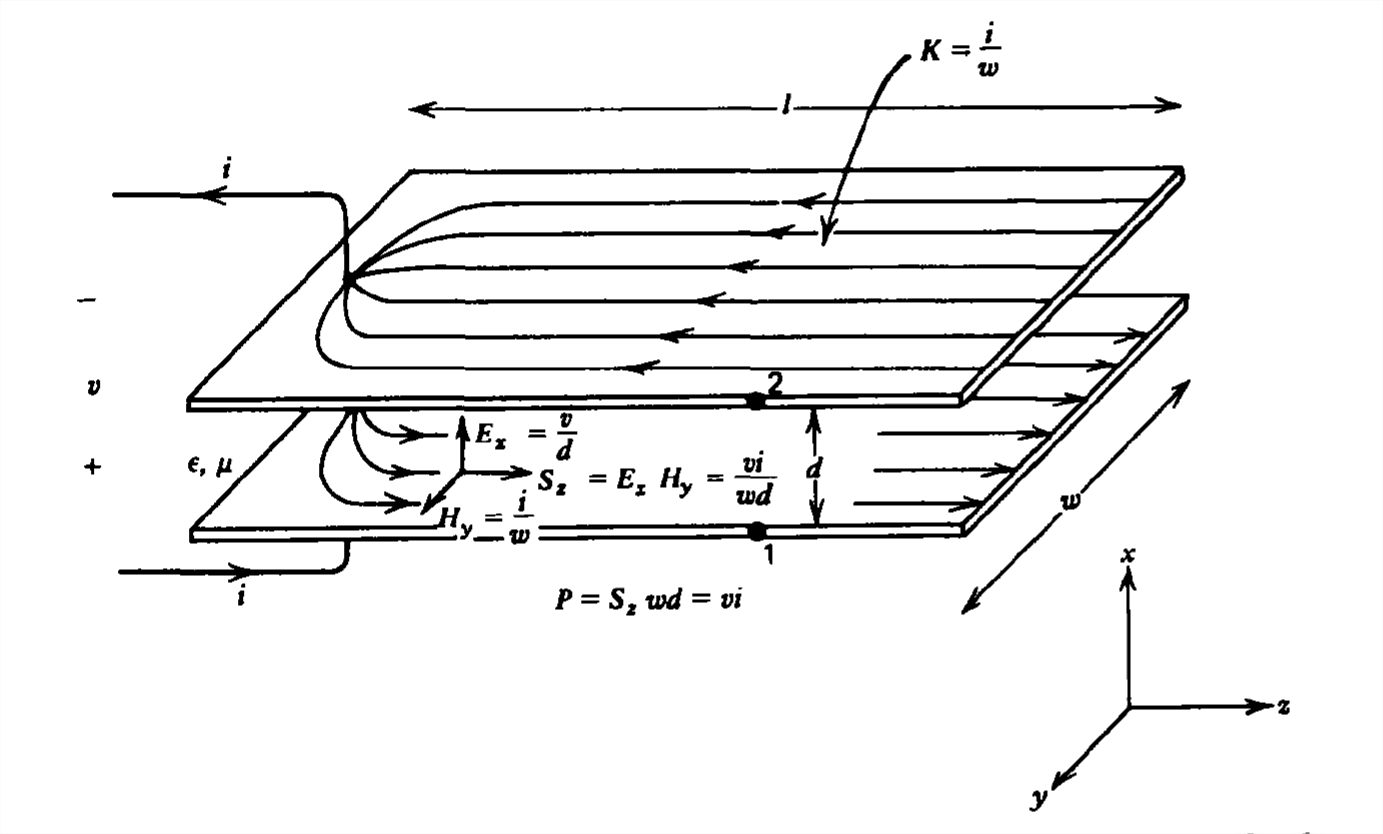
The general properties of transmission lines are illustrated in Figure 8-1 by the parallel plate electrodes a small distance d apart enclosing linear media with permittivity \(\varepsilon \) and permeability \(\mu \). Because this spacing \( d\) is much less than the width \(w\) or length \(l\), we neglect fringing field effects and assume that the fields only depend on the \( z\) coordinate.

The perfectly conducting electrodes impose the boundary conditions:

(i)    The tangential component of \(\textbf{E}\) is zero.
(ii)    The normal component of \(\textbf{B}\) (and thus \(\textbf{H}\) in the linear media) is zero.

With these constraints and the, neglect of fringing near the electrode edges, the fields cannot depend on \(x\) or \(y\) and thus are of the following form:

\[\textbf{E}=E_{x}\left ( z,t \right )\textbf{i}_x\\
\textbf{H}=H_{y}\left ( z,t \right )\textbf{i}_y \]

which when substituted into Maxwell's equations yield

Figure 8-1 The simplest transmission line consists of two parallel perfectly conducting plates a small distance \(d\) apart.

\[\nabla \times \textbf{E}=-\mu \frac{\partial \textbf{H}}{\partial t}\Rightarrow \frac{\partial E_{x}}{\partial z}=-\mu \frac{\partial H_{y}}{\partial t}\\\nabla \times \textbf{H}=\varepsilon  \frac{\partial \textbf{E}}{\partial t}\Rightarrow \frac{\partial H_{y}}{\partial z}=-\varepsilon \frac{\partial E_{x}}{\partial t} \]

We recognize these equations as the same ones developed for plane waves in Section 7-3-1. The wave solutions found there are also valid here. However, now it is more convenient to introduce the circuit variables of voltage and current along the transmission line, which will depend on \(z\) and \(t\).

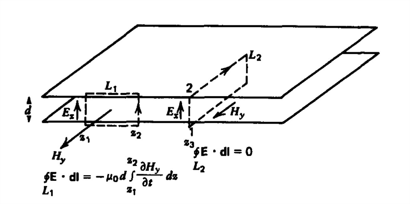
Kirchoff's voltage and current laws will not hold along the transmission line as the electric field in (2) has nonzero curl and the current along the electrodes will have a divergence due to the time varying surface charge distribution, \(\sigma _{f}=\pm \varepsilon E_{x}\left ( z,t \right )\). Because \(\textbf{E}\) has a curl, the voltage difference measured between any two points is not unique, as illustrated in Figure 8-2, where we see time-varying magnetic flux passing through the contour \(L_{1}\). However, no magnetic flux passes through the path \(L_{2}\), where the potential difference is measured between the two electrodes at the same value of \(z\), as the magnetic flux is parallel to the surface. Thus, the voltage can be uniquely defined between the two electrodes at the same value of \(z\):

\[v\left ( z,t \right )=\underset{\textrm{z=const}}{\int_{1}^{2}}\textbf{E}\cdot \textbf{dl}=E_{x}\left ( z,t \right )d \]

Figure 8-2 The potential difference measured between any two arbitrary points at different positions \(z_{1}\) and \(z_{2}\) on the transmission line is not unique-the line integral \(L_{1}\)L, of the electric field is nonzero since the contour has magnetic flux passing through it. If the contour \(L_{2}\) lies within a plane of constant \(z\) such as at \(z_{3}\), no magnetic flux passes through it so that the voltage difference between the two electrodes at the same value of \(z\) is unique.

Similarly, the tangential component of \(\textbf{H}\) is discontinuous at each plate by a surface current \(\pm \textbf{K}\). Thus, the total current \(i\left ( z,t \right )\) flowing in the \(z\) direction on the lower plate is

\[i\left ( z,t \right )=K_{z}w=H_{y}w \]

Substituting (3) and (4) back into (2) results in the transmission line equations:

\[\frac{\partial v}{\partial z}=-L\frac{\partial i}{\partial t} \]

where \(L\) and \(C\) are the inductance and capacitance per unit length of the parallel plate structure:

\[L=\frac{\mu d}{w}\,\textrm{henry/m}\quad C=\frac{\varepsilon w}{d}\,\textrm{farad/m} \]

If both quantities are multiplied by the length of the line \(l\), we obtain the inductance of a single turn plane loop if the line were short circuited, and the capacitance of a parallel plate capacitor if the line were open circuited.

It is no accident that the \(LC\) product

\[LC=\varepsilon \mu =1/c^{2} \]

is related to the speed of light in the medium.

General Transmission Line Structures

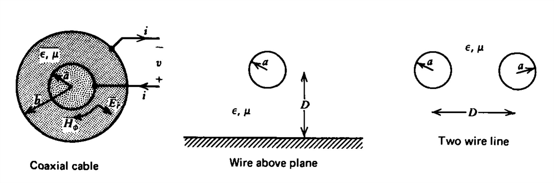
The transmission line equations of (5) are valid for any two-conductor structure of arbitrary shape in the transverse \(xy\) plane but whose cross-sectional area does not change along its axis in the \(z\) direction. \(L\) and \(C\) are the inductance and capacitance per unit length as would be calculated in the quasi-static limits. Various simple types of transmission lines are shown in Figure 8-3. Note that, in general, the field equations of (2) must be extended to allow for \(x\) and \(y\) components but still no \(z\) components:

\[\textbf{E}=\textbf{E}_{T}\left ( x,y,z,t \right )=E_{x}\textbf{i}_{x}+E_{y}\textbf{i}_{y},\quad E_z=0\\
\textbf{H}=\textbf{H}_{T}\left ( x,y,z,t \right )=H_{x}\textbf{i}_{x}+H_{y}\textbf{i}_{y},\quad H_z=0 \]

We use the subscript \(T\) in (8) to remind ourselves that the fields lie purely in the transverse \(xy\) plane. We can then also distinguish between spatial derivatives along the \(z\) axis \(\left ( \partial/\partial z\right )\) from those in the transverse plane \(\left ( \partial/\partial x, \partial/\partial y\right ) \):

\[\nabla\underbrace{=\nabla_{T}}_{\textbf{i}_{x}\frac{\partial }{\partial x}+\textbf{i}_{y}\frac{\partial }{\partial y}}+\textbf{i}_{z}\frac{\partial }{\partial z} \]

We may then write Maxwell's equations as

\[\begin{align}\nabla_T\times \textbf{E}_{T}+\frac{\partial }{\partial z}\left (\textbf{i}_{z}\times \textbf{E}_{T} \right )&=-\mu \frac{\partial \textbf{H}_{T}}{\partial t} \\
\nabla_T\times \textbf{H}_{T}+\frac{\partial }{\partial z}\left (\textbf{i}_{z}\times \textbf{H}_{T} \right )&=-\varepsilon  \frac{\partial \textbf{E}_{T}}{\partial t} \nonumber \\
\nabla_T\cdot \textbf{E}_{T}&=0 \nonumber \\
\nabla_T\cdot \textbf{H}_{T}&=0 \nonumber \end{align} \]

The following vector properties for the terms in (10) apply:

1. \(\nabla_T\times \textbf{H}_{T}\) and \(\nabla_T\times \textbf{E}_{T}\) lie purely in the \(z\) direction.
2. \(\textbf{i}_{z}\times \textbf{E}_{T}\) and \(\textbf{i}_{z}\times \textbf{H}_{T}\) lie purely in the \(xy\) plane.

Figure 8-3 Various types of simple transmission lines.

Thus, the equations in (10) may be separated by equating vector components:

\begin{align}
\nabla_T\times \textbf{E}_{T}&=0,\quad \nabla_T\times \textbf{H}_{T}=0 \\
\nabla_T\cdot  \textbf{E}_{T}&=0,\quad \nabla_T\cdot  \textbf{H}_{T}=0 \nonumber \\
\frac{\partial }{\partial z}\left ( \textbf{i}_{z}\times \textbf{E}_{T} \right )&=-\mu \frac{\partial \textbf{H}_{T}}{\partial t}\Rightarrow \frac{\partial \textbf{E}_{T}}{\partial z}=\mu \frac{\partial }{\partial t}\left ( \textbf{i}_{z}\times \textbf{H}_{T} \right ) \\
\frac{\partial }{\partial z}\left ( \textbf{i}_{z}\times \textbf{H}_{T} \right )&=\varepsilon  \frac{\partial \textbf{E}_{T}}{\partial t}
\nonumber \end{align}

where the Faraday's law equalities are obtained by crossing with \( \textbf{i}_{z}\), and expanding the double cross product

\[\textbf{i}_{z}\times \left ( \textbf{i}_{z}\times \textbf{E}_{T} \right )= \textbf{i}_{z}\left ( \textbf{i}_{z} \underset{\nearrow \quad }{\overset{\qquad 0}{\overset{\quad \nearrow}{\cdot}}} \textbf{E}_{T} \right ) -\textbf{E}_{T}\left ( \textbf{i}_{z}\cdot \textbf{i}_{z} \right )=-\textbf{E}_{T}  \]

and remembering that \(\textbf{i}_{z}\cdot \textbf{E}_{T}\).

The set of equations in (11) tell us that the field dependences on the transverse coordinates are the same as if the system were static and source free. Thus, all the tools developed for solving static field solutions, including the two-dimensional Laplace's equations and the method of images, can be used to solve for \(\textbf{E}_{T}\) and \(\textbf{H}_{T}\) in the transverse \(xy\) plane.

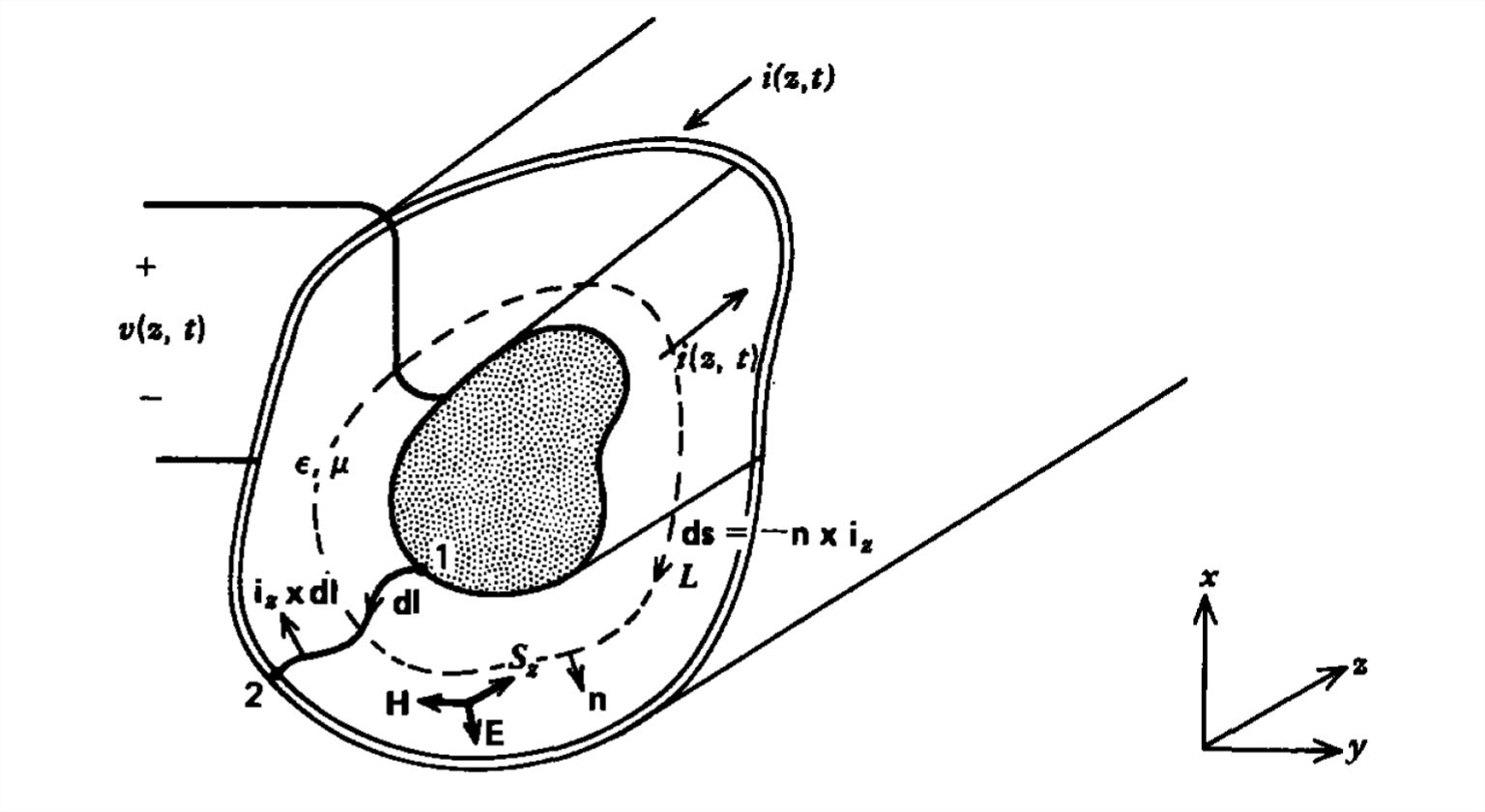
We need to relate the fields to the voltage and current defined as a function of \(z\) and \(t\) for the transmission line of arbitrary shape shown in Figure 8-4 as

\[v\left ( z,t \right )=\underset{\textrm{z=const}}{\int_{1}^{2}}\textbf{E}_{T}\cdot \textbf{dl}\\
i\left ( z,t \right ) = \oint_{\textrm{contour}\,L\\
\textrm{at constant}\, z \\
\textrm{enclosing the}\\
\textrm{inner conductor}}\textbf{H}_{T}\cdot \textbf{dl} \]

The related quantities of charge per unit length \(\)q and flux per unit length \(\)A along the transmission line are

\[q\left ( z,t \right )=\varepsilon \underset{\textrm{z=const}}{\oint_{L}}\textbf{E}_{T}\cdot \textbf{n}\,dS\\
\lambda \left ( z,t \right ) = \mu \underset{\textrm{z=const}}{\int_{1}^{2}}\textbf{H}_{T}\cdot \left (\textbf{i}_{z} \times  \textbf{dl}\right ) \]

The capacitance and inductance per unit length are then defined as the ratios:

\[C=\frac{q\left ( z,t \right )}{v\left ( z,t \right )}=\frac{\varepsilon \oint_{L}\textbf{E}_{T}\cdot \textbf{dS}}{\int_{1}^{2}\textbf{H}_{T}\cdot \textbf{dl}}\Big|_{\textrm{z=const}}\\
L=\frac{\lambda \left ( z,t \right )}{i\left ( z,t \right )}=\frac{\mu \int_{1}^{2}\textbf{H}_{T}\cdot \left (\textbf{i}_{z} \times  \textbf{dl}\right )}{\oint_{L}\textbf{H}_{T}\cdot \textbf{dS}}\Big|_{\textrm{z=const}} \]

Figure 8-4 A general transmission line has two perfect conductors whose cross-sectional area does not change in the direction along its \(z\) axis, but whose shape in the transverse \(xy\) plane is arbitrary. The electric and magnetic fields are perpendicular, lie in the transverse \(xy\) plane, and have the same dependence on \(x\) and \(y\) as if the fields were static.

which are constants as the geometry of the transmission line does not vary with \(z\). Even though the fields change with \(z\), the ratios in (16) do not depend on the field amplitudes.

To obtain the general transmission line equations, we dot the upper equation in (12) with \(\textbf{dl}\), which can be brought inside the derivatives since \(\textbf{dl}\) only varies with \(x\) and \(y\) and not \(z\) or \(t\). We then integrate the resulting equation over a line at constant \(z\) joining the two electrodes:

\[\begin{align}\frac{\partial }{\partial z} \left ( \int_{1}^{2}\textbf{E}_{T}\cdot \textbf{dl} \right )&=\frac{\partial }{\partial t}\left ( \mu \int_{1}^{2}\left ( \textbf{i}_{z}\times \textbf{H}_{T} \right )\cdot \textbf{dl} \right ) \\ &=-\frac{\partial }{\partial t}\left ( \mu \int_{1}^{2} \textbf{H}_{T}\times \left (\textbf{i}_{z} \cdot \textbf{dl}\right ) \right ) \nonumber \end{align}  \]

where the last equality is obtained using the scalar triple product allowing the interchange of the dot and the cross:

\[\left ( \textbf{i}_{z}\times \textbf{H}_{T} \right )\cdot \textbf{dl}=-\left ( \textbf{H}_{T}\times \textbf{i}_{z} \right )\cdot \textbf{dl}=-\textbf{H}_{T} \cdot \left ( \textbf{i}_{z}\times\textbf{dl} \right )  \]

We recognize the left-hand side of (17) as the \(z\) derivative of the voltage defined in (14), while the right-hand side is the negative time derivative of the flux per unit length defined in (15):

\[\frac{\partial v}{\partial z} =-\frac{\partial \lambda }{\partial t} =-L\frac{\partial i}{\partial t}  \]

We could also have derived this last relation by dotting the upper equation in (12) with the normal \(\textbf{n}\) to the inner conductor and then integrating over the contour \(L\) surrounding the inner conductor:

\[\frac{\partial }{\partial z} \left ( \oint _L \textbf{n}\cdot \textbf{E}_{T}ds \right )=\frac{\partial }{\partial t}\left ( \mu \oint _L \textbf{n}\cdot \left ( \textbf{i}_{z}\times \textbf{H}_{T} \right )ds \right )=-\frac{\partial }{\partial t}\left ( \mu \oint _L \textbf{H}_{T}\cdot \textbf{ds} \right )  \]

where the last equality was again obtained by interchanging the dot and the cross in the scalar triple product identity:

\[\textbf{n}\cdot \left ( \textbf{i}_{z}\times \textbf{H}_{T} \right )=\left ( \textbf{n}\times \textbf{i}_{z}\right )\cdot  \textbf{H}_{T} =-\textbf{H}_{T}\cdot \textbf{ds} \]

The left-hand side of (20) is proportional to the charge per unit length defined in (15), while the right-hand side is proportional to the current defined in (14):

\[\frac{1}{\varepsilon }\frac{\partial q}{\partial z}=-\mu \frac{\partial i}{\partial t}\Rightarrow C\frac{\partial v}{\partial z}=-\varepsilon \mu \frac{\partial i}{\partial t} \]

Since (19) and (22) must be identical, we obtain the general result previously obtained in Section 6-5-6 that the inductance and capacitance per unit length of any arbitrarily shaped transmission line are related as

\[LC=\varepsilon \mu  \]

We obtain the second transmission line equation by dotting the lower equation in (12) with \(\textbf{dl}\) and integrating between electrodes:

\[\frac{\partial }{\partial t} \left ( \varepsilon \int_{1}^{2} \textbf{E}_{T}\cdot \textbf{dl} \right )=\frac{\partial }{\partial z}\left (\int_{1}^{2}\left ( \textbf{i}_{z}\times \textbf{H}_{T} \right )\cdot \textbf{dl} \right )=-\frac{\partial }{\partial z}\left (\int_{1}^{2} \textbf{H}_{T}\cdot\left ( \textbf{i}_z \times \textbf{dl}\right )\right ) \]

to yield from (14)-(16) and (23)

\[\varepsilon \frac{\partial v}{\partial t}=-\frac{1}{\mu }\frac{\partial \lambda }{\partial z}=-\frac{L}{\mu }\frac{\partial i}{\partial z}\Rightarrow \frac{\partial i}{\partial z}=-C\frac{\partial v}{\partial t} \]

Example \(\PageIndex{1}\) EXAMPLE 8-1 THE COAXIAL TRANSMISSION LINE

Consider the coaxial transmission line shown in Figure 8-3 composed of two perfectly conducting concentric cylinders of radii \(a\) and \(b\) enclosing a linear medium with permittivity \(\varepsilon \) and permeability \(\mu \). We solve for the transverse dependence of the fields as if the problem were static, independent of time. If the voltage difference between cylinders is \(v\) with the inner cylinder carrying a total current \(i\) the static fields are

\(E_{r}=\frac{v}{\textrm{r}\ln \left ( b/a \right )},\quad H_{\phi }=\frac{i}{2\pi \textrm{r}}\)

The surface charge per unit length \(q\) and magnetic flux per unit length \(\lambda \) are

\(q=\varepsilon E_{r}\left ( \textrm{r}=a \right )2\pi a=\frac{2\pi \varepsilon v}{\ln \left ( b/a \right )}\\
\lambda =\int_{a}^{b}\mu H_{\phi }d\textrm{r}=\frac{\mu i}{2\pi }\ln \frac{b}{a}\)

so that the capacitance and inductance per unit length of this structure are

\(C=\frac{q}{v}=\frac{2\pi \varepsilon}{\ln \left ( b/a \right )},\quad L=\frac{\lambda }{i}=\frac{\mu }{2\pi }\ln \frac{b}{a}\)

where we note that as required

\(LC=\varepsilon \mu \)

Substituting \(E_r\) and \(H_{\phi }\) into (12) yields the following transmission line equations:

\(\frac{\partial E_{r}}{\partial z}=-\mu \frac{\partial H_{\phi }}{\partial t}\Rightarrow \frac{\partial v}{\partial z}=-L\frac{\partial i}{\partial t}\\
\frac{\partial H_{\phi }}{\partial z}=-\varepsilon \frac{\partial E_{r}}{\partial t}\Rightarrow \frac{\partial i}{\partial z}=-C\frac{\partial v}{\partial t}\)

Distributed Circuit Representation

Thus far we have emphasized the field theory point of view from which we have derived relations for the voltage and current. However, we can also easily derive the transmission line equations using a distributed equivalent circuit derived from the following criteria:

1.     The flow of current through a lossless medium between two conductors is entirely by displacement current, in exactly the same way as a capacitor.
2.     The flow of current along lossless electrodes generates a magnetic field as in an inductor.

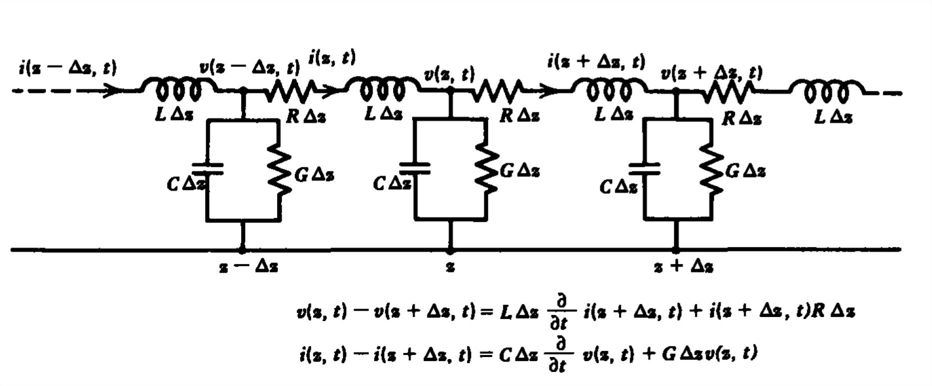
Thus, we may discretize the transmission line into many small incremental sections of length \(\Delta z\) with series inductance \(L\,\Delta z\) and shunt capacitance \(C\,\Delta z\), where \(L\) and \(C\) are the inductance and capacitance per unit lengths. We can also take into account the small series resistance of the electrodes \(R\,\Delta z\), where \(R\) is the resistance per unit length (ohms per meter) and the shunt conductance loss in the dielectric \(\)G Az, where \(\)G is the conductance per unit length (siemens per meter). If the transmission line and dielectric are lossless, \R =0(\), \(G =0\).

The resulting equivalent circuit for a lossy transmission line shown in Figure 8-5 shows that the current at \(z+\Delta z\) and \(z\) differ by the amount flowing through the shunt capacitance and conductance:

\[i\left ( z,t \right )-i\left ( z+\Delta z,t \right )=C\Delta z\frac{\partial v\left ( z,t \right )}{\partial t}+G\Delta z\,v\left ( z,t \right ) \]

Similarly, the voltage difference at \(z+\Delta z\) from \(z\) is due to the drop across the series inductor and resistor:

\[v\left ( z,t \right )-v\left ( z+\Delta z,t \right )=L\Delta z\frac{\partial i\left ( z+\Delta z,t \right )}{\partial t}+i\left ( z+\Delta z,t \right )R\,\Delta z \]

By dividing (26) and (27) through by \(\Delta z\) and taking the limit as \(\Delta z\rightarrow 0\), we obtain the lossy transmission line equations:

\[\lim_{\Delta z\rightarrow 0}\frac{i\left ( z+\Delta z,t \right )-i\left ( z,t \right )}{\Delta z}=\frac{\partial i}{\partial z}=-C\frac{\partial v}{\partial t}-Gv\\
\lim_{\Delta z\rightarrow 0}\frac{v\left ( z+\Delta z,t \right )-v\left ( z,t \right )}{\Delta z}=\frac{\partial v}{\partial z}=-L\frac{\partial i}{\partial t}-iR \]

which reduce to (19) and (25) when \(R\) and \(G\) are zero.

Power Flow

Multiplying the upper equation in (28) by \(v\) and the lower by \(i\) and then adding yields the circuit equivalent form of Poynting's theorem:

\[\frac{\partial }{\partial z}\left ( vi \right )=-\frac{\partial }{\partial t}\left ( \frac{1}{2}Cv^{2}+\frac{1}{2}Li^{2} \right )-Gv^{2}-i^{2}R \]

Figure 8-5 Distributed circuit model of a transmission line including small series and shunt resistive losses.

The power flow \(vi\) is converted into energy storage \(\left ( \frac{1}{2}Cv^{2}+\frac{1}{2}Li^{2} \right )\) or is dissipated in the resistance and conductance per unit lengths.

From the fields point of view the total electromagnetic power flowing down the transmission line at any position \(z\) is

\[P\left ( z,t \right )=\int_{\textbf{S}}\left ( \textbf{E}_{T}\times \textbf{H}_{T} \right )\cdot \textbf{i}_{z}d\textrm{S}=\int_{\textbf{S}}\textbf{E}_{T}\cdot \left ( \textbf{H}_{T}\times \textbf{i}_{z}  \right )d\textrm{S} \]

where \(\textrm{S}\) is the region between electrodes in Figure 8-4. Because the transverse electric field is curl free, we can define the scalar potential

\[\nabla \times \textbf{E}_{T}=0\Rightarrow \textbf{E}_{T}=-\nabla_{T}V \]

so that (30) can be rewritten as

\[P\left ( z,t \right )=\int_{\textbf{S}}\left ( \textbf{i}_{z}\times \textbf{H}_{T} \right )\cdot \nabla_{T}Vd\textrm{S} \]

It is useful to examine the vector expansion

\[\nabla_{T}\cdot \left [ V\left ( \textbf{i}_{z}\times \textbf{H}_{T} \right ) \right ]=\left ( \textbf{i}_{z}\times \textbf{H}_{T} \right )\cdot \nabla_{T}V+V\nabla_{T}\cdot \left ( \textbf{i}_{z} \underset{\nearrow \quad }{\overset{\qquad 0}{\overset{\quad \nearrow}{\times }}} \textbf{E}_{T} \right ) \]

where the last term is zero because \(\textbf{i}_{z}\) is a constant vector and \(\textbf{H}_{T}\) is also curl free:

\[\nabla_{T}\cdot \left ( \textbf{i}_{z}\times \textbf{H}_{T} \right )=\textbf{H}_{T}\cdot \left ( \nabla_{T}\times \textbf{i}_{z} \right )-\textbf{i}_{z}\cdot \left ( \nabla_{T}\times \textbf{H}_{T} \right )=0 \]

Then (32) can be converted to a line integral using the two-dimensional form of the divergence theorem:

\begin{align} P\left ( z,t \right )& =\int_{\textbf{S}}\nabla_{T}\cdot \left [ V\left ( \textbf{i}_{z}\times \textbf{H}_{T} \right ) \right ]d\textrm{S} \\ &
=\underset{\textrm{contours on}\\ \textrm{the surface of}\\ \textrm{both electrodes}}{-\int}V\left ( \textbf{i}_{z}\times \textbf{H}_{T} \right )\cdot \textbf{n}\,ds \nonumber \end{align}

where the line integral is evaluated at constant \(z\) along the surface of both electrodes. The minus sign arises in (35) because \(\textbf{n}\) is defined inwards in Figure 8-4 rather than outwards as is usual in the divergence theorem. Since we are free to pick our zero potential reference anywhere, we take the outer conductor to be at zero voltage. Then the line integral in (35) is only nonzero over the inner conductor, where \(V=v\):

\begin{align}P\left ( z,t \right ) &=\underset{\textrm{inner}\\\textrm{conductor}}{-v\oint}\left (\textbf{i}_{z}\times \textbf{H}_{T} \right )\cdot \textbf{n}ds \\ &
=\underset{\textrm{inner}\\\textrm{conductor}}{v\oint }\left ( \textbf{H}_{T}\times \textbf{i}_{z}\right )\cdot \textbf{n}ds \nonumber \\ &
=\underset{\textrm{inner}\\\textrm{conductor}}{v\oint } \textbf{H}_{T}\cdot \left (\textbf{i}_{z}\times \textbf{n}\right )ds \nonumber \\ &
=\underset{\textrm{inner}\\\textrm{conductor}}{v\oint }\textbf{H}_{T}\textbf{dS} \nonumber \\ &
=vi \nonumber \end{align} 

where we realized that \(\left (\textbf{i}_{z}\times \textbf{n}\right )ds= \textbf{ds}\), defined in Figure 8-4 if \(L\) lies along the surface of the inner conductor. The electromagnetic power flowing down a transmission line just equals the circuit power.

The Wave Equation

Restricting ourselves now to lossless transmission lines so that \(R = G =0\) in (28), the two coupled equations in voltage and current can be reduced to two single wave equations in \(v\) and \(i\):

\[\frac{\partial^2 v}{\partial t^2}=c^{2}\frac{\partial^2 v}{\partial z^2}\\
\frac{\partial^2 i}{\partial t^2}=c^{2}\frac{\partial^2 i}{\partial z^2} \]

where the speed of the waves is

\[c=\frac{1}{\sqrt{LC}}=\frac{1}{\sqrt{\varepsilon \mu }}\,\textrm{m/sec}  \]

As we found in Section 7-3-2 the solutions to (37) are propagating waves in the \(\pm z\) directions at the speed \(c\):

\[v\left ( z,t \right )=\textrm{V}_{+}\left ( t-z/c \right )+\textrm{V}_{-}\left ( t+z/c \right )\\
i\left ( z,t \right )=I_{+}\left ( t-z/c \right )+I_{-}\left ( t+z/c \right ) \]

where the functions \(\textrm{V}_{+}\), \(\textrm{V}_{-}\), \(I_{+}\), and \(I_{-}\) are determined by boundary conditions imposed by sources and transmission line terminations. By substituting these solutions back into
(28) with \(R = G = 0\), we find the voltage and current functions related as

\[\textrm{V}_{+}=I_{+}Z_{0}\\
\textrm{V}_{-}=-I_{-}Z_{0} \]

where

\[Z_{0}=\sqrt{L/C}\,\textrm{ohm} \]

is known as the characteristic impedance of the transmission line, analogous to the wave impedance \(\eta \) in Chapter 7. Its inverse \(Y_{0}=1/Z_{0}\) is also used and is termed the characteristic admittance. In practice, it is difficult to measure \(L\) and \(C\) of a transmission line directly. It is easier to measure the wave speed \(c\) and characteristic impedance \(Z_{0}\) and then calculate \(L\) and \(C\) from (38) and (41).

The most useful form of the transmission line solutions of (39) that we will use is

\[v\left ( z,t \right )=\textrm{V}_{+}\left ( t-z/c \right )+\textrm{V}_{-}\left ( t+z/c \right )\\
i\left ( z,t \right )=Y_{0}\left [\textrm{V}_{+}\left ( t-z/c \right )-\textrm{V}_{-}\left ( t+z/c \right )\right ] \]

Note the complete duality between these voltage-current solutions and the plane wave solutions in Section 7-3-2 for the electric and magnetic fields.