8.2: Transmission Line Transient Waves

The easiest way to solve for transient waves on transmission lines is through use of physical reasoning as opposed to mathematical rigor. Since the waves travel at a speed \(c\), once generated they cannot reach any position \(z\) until a time \(z/c\) later. Waves traveling in the positive \(z\) direction are described by the function \(\textrm{V}_{+}\left ( t-z/c \right )\) and waves traveling in the \(-z\) direction by \(\textrm{V}_{-}(t + z/c)\). However, at any time \(t\) and position \(z\), the voltage is equal to the sum of both solutions while the current is proportional to their difference.

Transients on Infinitely Long Transmission Lines

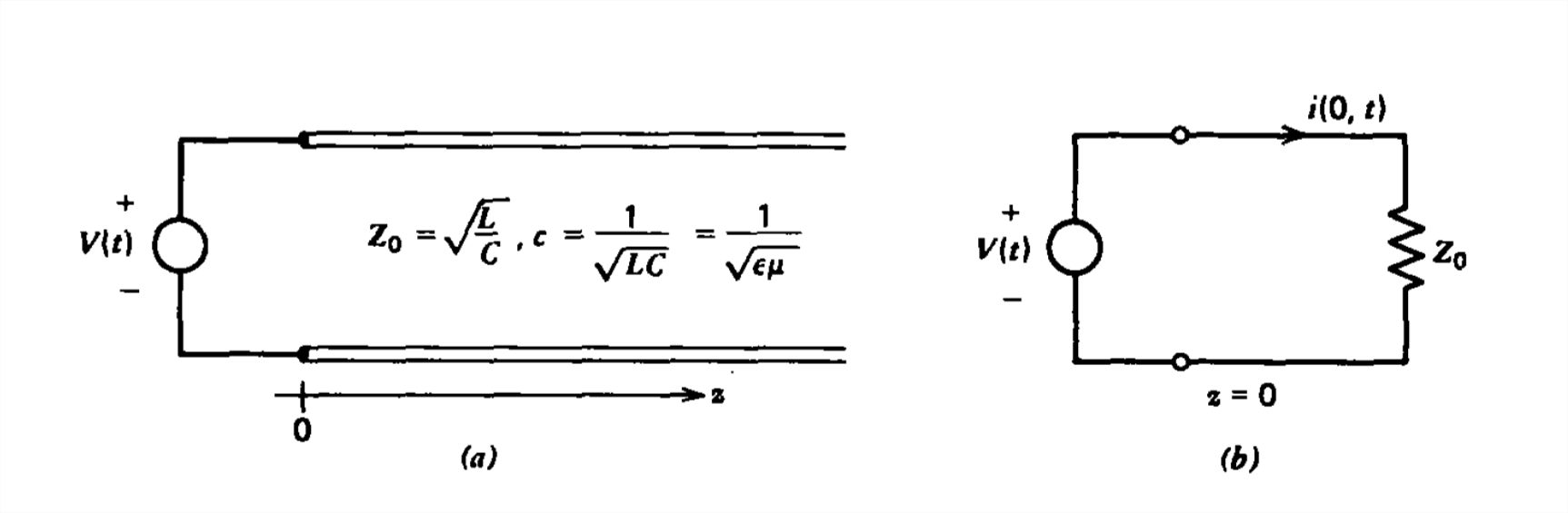
The transmission line shown in Figure 8-6a extends to infinity in the positive \(z\) direction. A time varying voltage source \(V(t)\) that is turned on at \(t =0\) is applied at \(z =0\) to the line which is initially unexcited. A positively traveling wave \(\textrm{V}_{+}\left ( t-z/c \right )\) propagates away from the source. There is no negatively traveling wave, \(\textrm{V}_{-}\left ( t-z/c \right )=0\). These physical

Figure 8-6 (a) A semi-infinite transmission line excited by a voltage source at \(z = 0\). (b) To the source, the transmission line looks like a resistor \(Z_{0}\) equal to the characteristic impedance. (c) The spatial distribution of the voltage \(v(z, t)\) at various times for a staircase pulse of \(V(t)\). (d) If the voltage source is applied to the transmission line through a series resistance \(R_{s}\) the voltage across the line at \(z=0\) is given by the voltage divider relation.

arguments are verified mathematically by realizing that at \(t =0\) the voltage and current are zero for \(z >0\),

\[ v\left ( z,t=0 \right )=\textrm{V}_{+}\left (-z/c \right )+\textrm{V}_{-}\left (-z/c \right )=0\\
i\left ( z,t=0 \right )=Y_{0}\left [  \textrm{V}_{+}\left (-z/c \right )+\textrm{V}_{-}\left (-z/c \right )\right ]=0  \]

which only allows the trivial solutions

\[ \textrm{V}_{+}\left (-z/c \right )=0,\quad  \textrm{V}_{-}\left (z/c \right )=0 \]

Since \(z\) can only be positive, whenever the argument of \(\textrm{V}_{+}\) is negative and of \(\textrm{V}_{-}\) positive, the functions are zero. Since \(t\) can only be positive, the argument of \(\textrm{V}_{-}\left (t +z/c \right )\) is always positive so that the function is always zero. The argument of \(\textrm{V}_{+}\left (t -z/c \right )\) can be positive, allowing a nonzero solution if \(t > z/c\) agreeing with our conclusions reached by physical arguments.

With \(\textrm{V}_{-}\left (t +z/c \right )=0\), the voltage and current are related as

\[ v\left ( z,t \right )=\textrm{V}_{+}\left (t -z/c \right )\\
i\left ( z,t \right )=Y_{0}\textrm{V}_{+}\left (t -z/c \right ) \]

The line voltage and current have the same shape as the source, delayed in time for any \(z\) by \(z/c\) with the current scaled in amplitude by \(Y_{0}\). Thus as far as the source is concerned, the transmission line looks like a resistor of value \(Z_{0}\) yielding the equivalent circuit at \(z =0\) shown in Figure 8-6b. At \(z =0\), the voltage equals that of the source

\[v\left ( 0,t \right )=\textrm{V}\left ( t \right )=\textrm{V}_{+}\left ( t \right ) \]

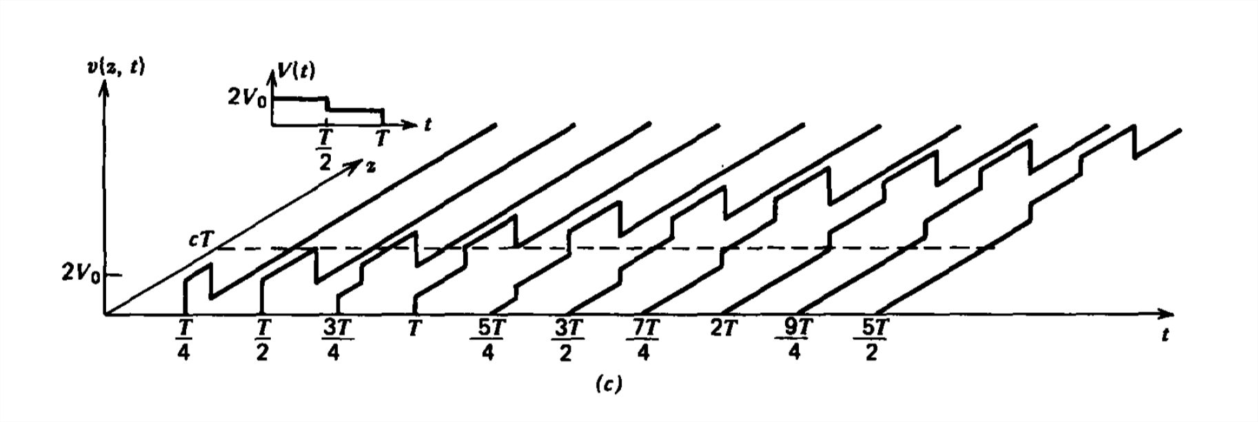
If \(V(t)\) is the staircase pulse of total duration \(T\) shown in Figure 8-6c, the pulse extends in space over the spatial interval:

\[ 0\leq z\leq ct,\quad 0\leq t\leq T\\
c\left ( t-T \right )\leq z\leq ct,\quad t> T \]

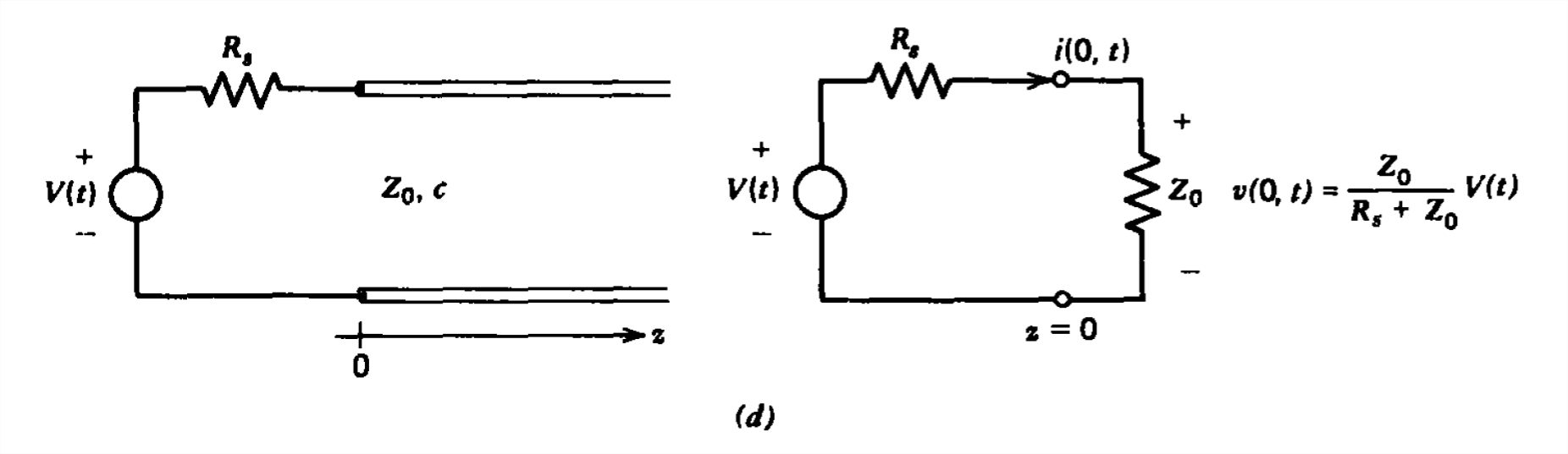
The analysis is the same even if the voltage source is in series with a source resistance \(R_s\), as in Figure 8-6d. At \(z =0\) the transmission line still looks like a resistor of value \(Z_0\) so that the transmission line voltage divides in the ratio given by the equivalent circuit shown:

\[ v\left ( z=0,t \right )=\frac{Z_{0}}{R_{s}+Z_{0}}\textrm{V}\left ( t \right )=\textrm{V}_{+}\left ( t \right )\\
i\left ( z=0,t \right )=Y_{0}\textrm{V}_{+}\left ( t \right )=\frac{\textrm{V}\left ( t \right )}{R_{s}+Z_{0}} \]

The total solution is then identical to that of (3) and (4) with the voltage and current amplitudes reduced by the voltage divider ratio \(Z_{0}/\left ( R_{s}+Z_{0} \right )\).

Reflections from Resistive Terminations

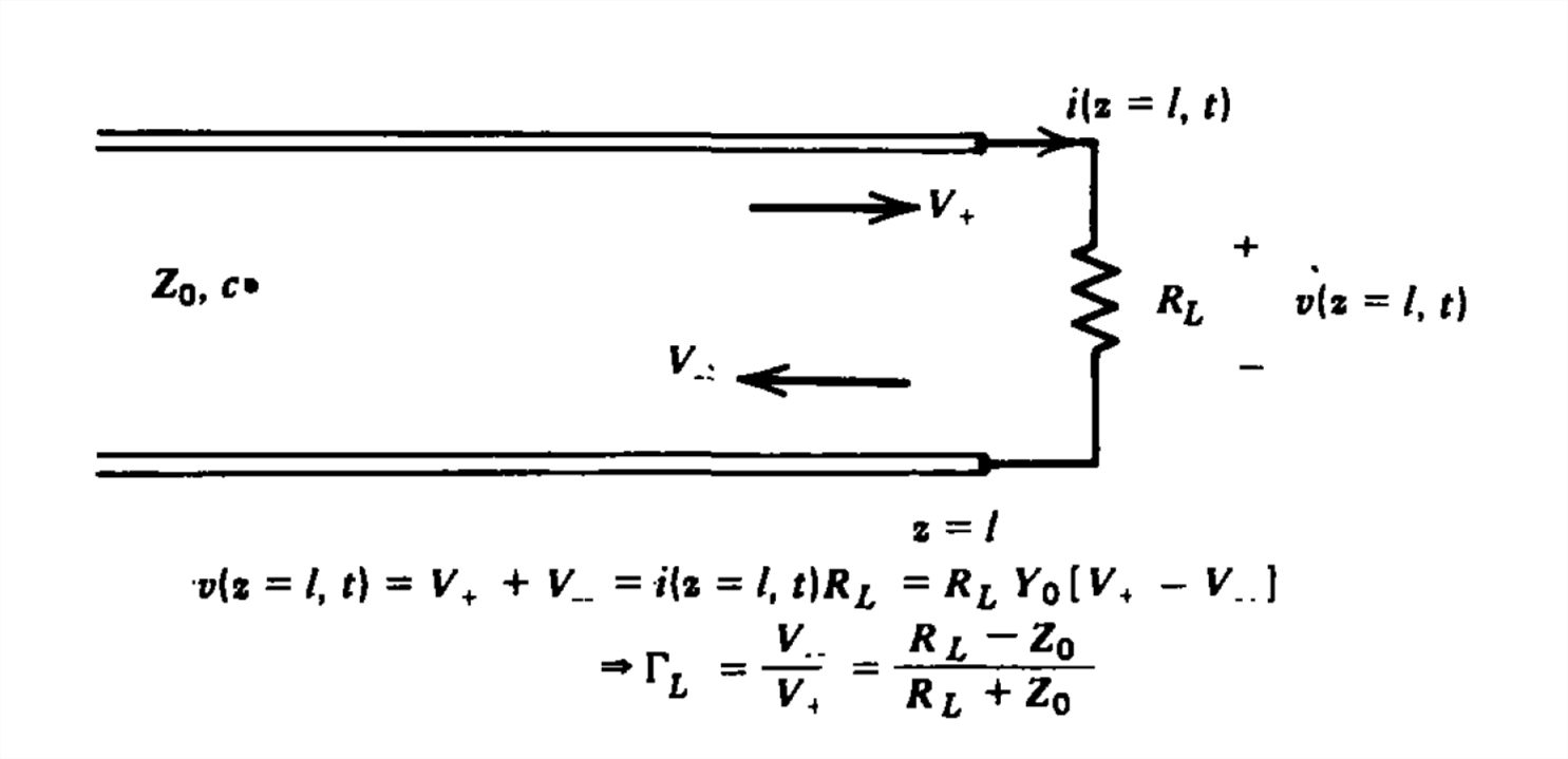
(a) Reflection Coefficient

All transmission lines must have an end. In Figure 8-7 we see a positively traveling wave incident upon a load resistor \(R_{L}\) at \(z = L\) The reflected wave will travel back towards the source at \(z =0\) as a \(\textrm{V}_{-}\) wave. At the \(z = l\) end the following circuit

Figure 8-7 A \(\textrm{V}_{+}\) wave incident upon the end of a transmission line with a load resistor \(R_{L}\) is reflected as a \(\textrm{V}_{-}\) wave.

relations hold:

\[ \begin{align} v\left ( l,t \right )&=\textrm{V}_{+}\left ( t-l/c \right )+\textrm{V}_{-}\left ( t+l/c \right ) \\ &
=i\left ( l,t \right )R_{L} \nonumber \\ &
=Y_{0}R_{L}\left [ \textrm{V}_{+}\left ( t-l/c \right )-\textrm{V}_{-}\left ( t+l/c \right ) \right ] \nonumber \end{align} \]

We then find the amplitude of the negatively traveling wave in terms of the incident positively traveling wave as

\[ \Gamma_{L} =\frac{\textrm{V}_{-}\left ( t+l/c \right )}{\textrm{V}_{+}\left ( t-l/c \right )}=\frac{R_{L}-Z_{0}}{R_{L}+Z_{0}} \]

where \(\Gamma_{L}\) is known as the reflection coefficient that is of the same form as the reflection coefficient \(R\) in Section 7-6-1 for normally incident uniform plane waves on a dielectric.

The reflection coefficient gives us the relative amplitude of the returning \(\textrm{V}_{-}\) wave compared to the incident \(\textrm{V}_{+}\) wave. There are several important limits of (8):

(i)    If \(R_{L}=Z_{0}\), the reflection coefficient is zero \(\left ( \Gamma _{0}=0 \right )\) so that there is no reflected wave and the line is said to be matched.
(ii)    If the line is short circuited \(\left ( R_{L}=0 \right )\), then \(\Gamma _{L}=-1\). The reflected wave is equal in amplitude but opposite in sign to the incident wave. In general, if \(R_{L}< Z_{0}\), the reflected voltage wave has its polarity reversed.
(iii)    If the line is open circuited \(\left ( R_{L}=\infty  \right )\), then \(\Gamma _{L}=+1\). The reflected wave is identical to the incident wave. In general, if \(R_{L}> Z_{0}\), the reflected voltage wave is of the same polarity as the incident wave.

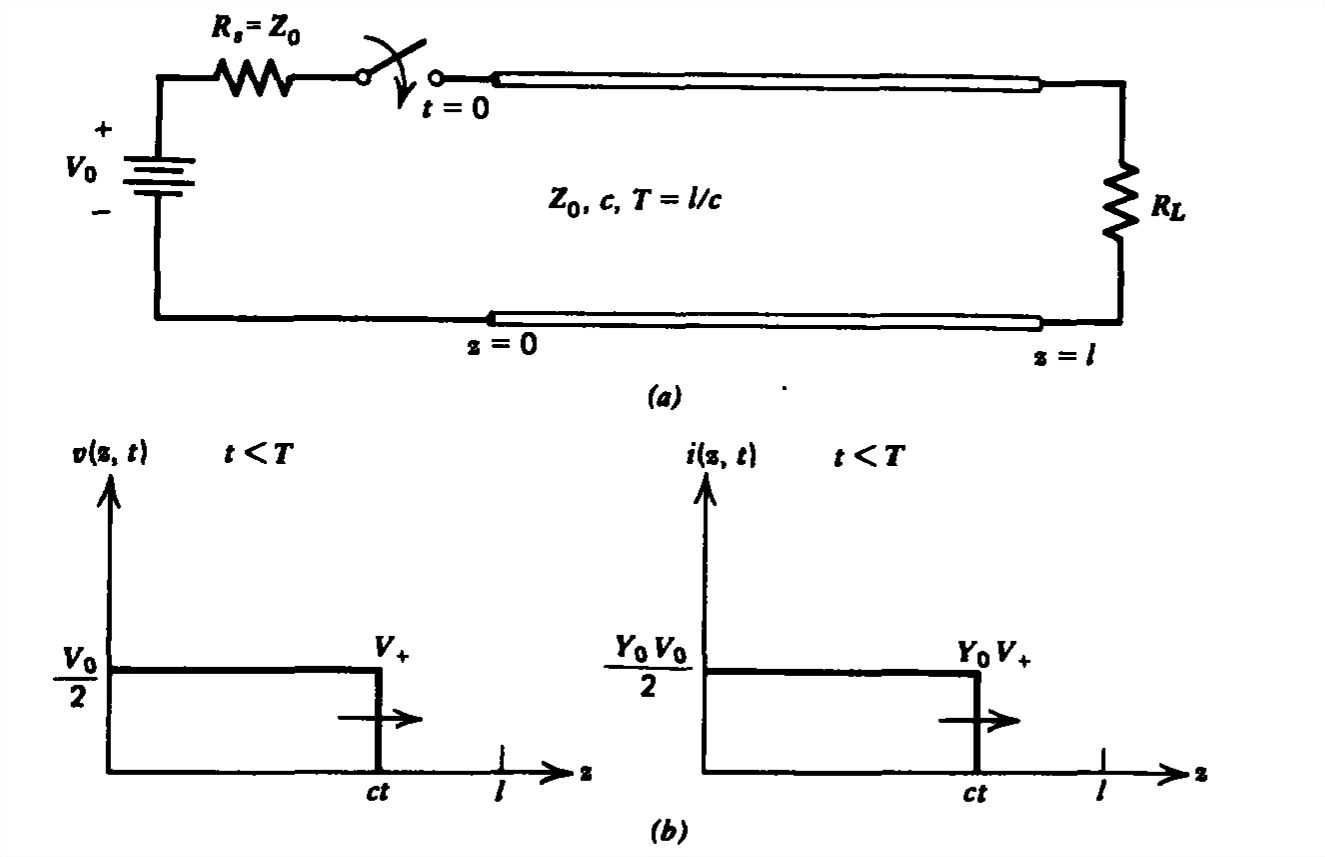
(b) Step Voltage

A dc battery of voltage \(V_{0}\) with series resistance \(R_{s}\), is switched onto the transmission line at \(t=0\), as shown in Figure 8-8a. At \(z =0\), the source has no knowledge of the

Figure 8-8 (a) A dc voltage \(V_{0}\) is switched onto a resistively loaded transmission line through a source resistance \(R_{s}\). (b) The equivalent circuits at \(z = 0\) and \(z =l\) allow us to calculate the reflected voltage wave amplitudes in terms of the incident waves.

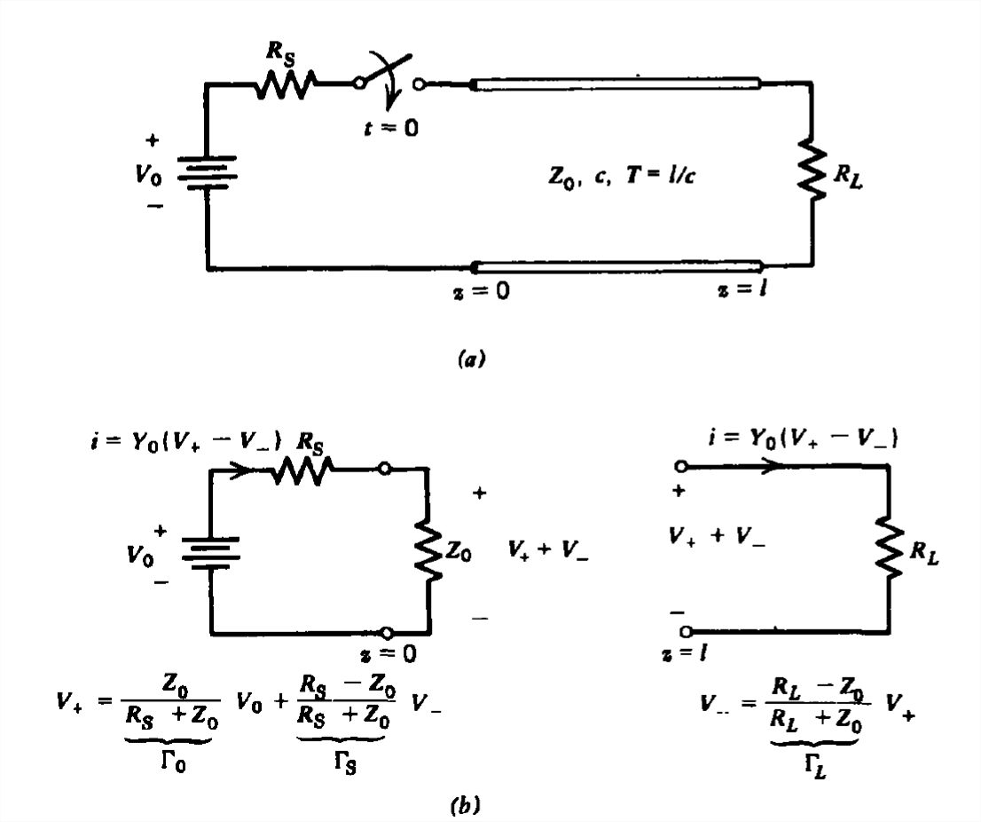
line's length or load termination, so as for an infinitely long line the transmission line looks like a resistor of value \(Z_{0}\) to the source. There is no \(\textrm{V}_{-}\) wave initially. The \(\textrm{V}_{+}\) wave is determined by the voltage divider ratio of the series source resistance and transmission line characteristic impedance as given by (6).

This \(\textrm{V}_{+}\) wave travels down the line at speed \(c\) where it is reflected at \(z = l\) for \(t > T\), where \(T = l/c\) is the transit time for a wave propagating between the two ends. The new \(\textrm{V}_{-}\) wave generated is related to the incident \(\textrm{V}_{+}\) wave by the reflection coefficient \(\Gamma _{L}\). As the \(\textrm{V}_{+}\) wave continues to propagate in the positive \(z\) direction, the \(\textrm{V}_{-}\) wave propagates back towards the source. The total voltage at any point on the line is equal to the sum of \(\textrm{V}_{+}\) and \(\textrm{V}_{-}\) while the current is proportional to their difference.

When the \(\textrm{V}_{-}\) wave reaches the end of the transmission line at \(z =0\) at time \(2T\), in general a new \(\textrm{V}_{+}\) wave is generated, which can be found by solving the equivalent circuit shown in Figure 8-8b:

\[ v\left ( 0,t \right )+i\left ( 0,t \right )R_{s} =V_{0}\Rightarrow \textrm{V}_{+}\left ( 0,t \right )+\textrm{V}_{-}\left ( 0,t \right )+ Y_{0}R_{s}\left [ \textrm{V}_{+}\left ( 0,t \right )-\textrm{V}_{-}\left ( 0,t \right ) \right ]=V_{0} \]

to yield

\[ \textrm{V}_{+}\left ( 0,t \right )=\Gamma _{s}\textrm{V}_{-}\left ( 0,t \right )+\frac{Z_{0}V_{0}}{Z_{0}+R_{s}},\quad \Gamma _{s}=\frac{R_{s}-Z_{0}}{R_{s}+Z_{0}} \]

where \(\Gamma _{s}\), is just the reflection coefficient at the source end. This new \(\textrm{V}_{+}\) wave propagates towards the load again generating a new \(\textrm{V}_{-}\) wave as the reflections continue.

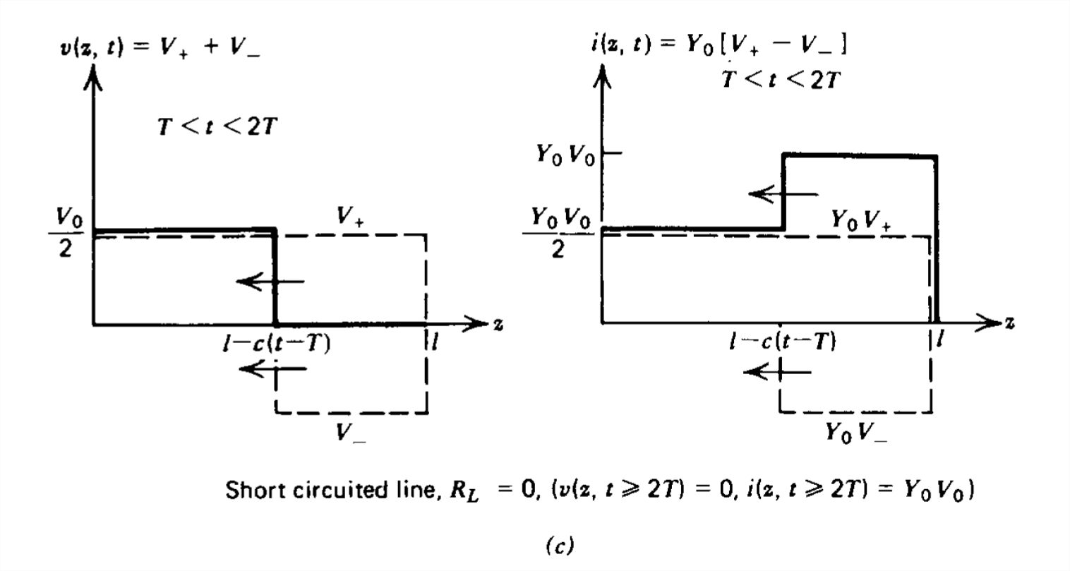
If the source resistance is matched to the line, \(R_{s}=Z_{0}\) so that \(\Gamma _{s}=0\), then \(\textrm{V}_{+}\) is constant for all time and the steady state is reached for \(t >2T\) If the load was matched, the steady state is reached for \(t>T\) no matter the value of \(R_{s}\). There are no further reflections from the end of a matched line. In Figure 8-9 we plot representative voltage and current spatial distributions for various times assuming the source is matched to the line for the load being matched, open, or short circuited.

(i) Matched Line

When \(R_{L}=Z_{0}\) the load reflection coefficient is zero so that \(\textrm{V}_{+}=V_{0}/2\) for all time. The wavefront propagates down the line with the voltage and current being identical in shape. The system is in the dc steady state for \(t\geq T\).

Figure 8-9 (a) A dc voltage is switched onto a transmission line with load resistance \(R_{L}\) through a source resistance \(R_{s}\) matched to the line. (b) Regardless of the load resistance, half the source voltage propagates down the line towards the load. If the load is also matched to the line \(\left ( R_{L}=Z_{0} \right )\), there are no reflections and the steady state of \(v\left ( z,t\geq T \right )=V_{0}/2,\quad i\left ( z,t\geq T \right )=Y_{0}V_{0}/2\) is reached for \(t\geq T\). (c) If the line is short circuited \(\left ( R_{L}=0 \right )\), then \(\Gamma _{L}=-1\) so that the \(\textrm{V}_{+}\) and \(\textrm{V}_{-}\) waves cancel for the voltage but add for the current wherever they overlap in space. Since the source end is matched, no further reflections arise at \(z = 0\) so that the steady state is reached for \(t\geq 2T\). (d) If the line is open circuited \(\left ( R_{L}=\infty  \right )\) so that \(\Gamma _{L}=\pm 1\), the \(\textrm{V}_{+}\)  and \(\textrm{V}_{-}\) waves add for the voltage but cancel for the current.

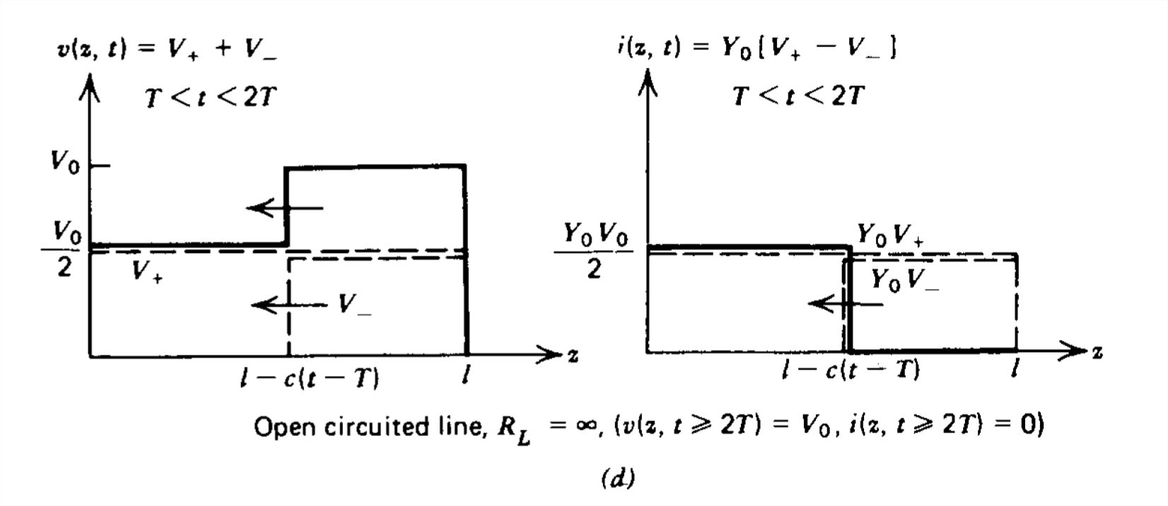
(ii) Open Circuited Line

When \(R_{L}=\infty\) the reflection coefficient is unity so that \(\textrm{V}_{+}=\textrm{V}_{-}\). When the incident and reflected waves overlap in space the voltages add to a stairstep pulse shape while the current is zero. For \(t\geq 2T\), the voltage is Vo everywhere on the line while the current is zero.

(iii) Short Circuited Line

When \(\left ( R_{L}=0 \right )\) the load reflection coefficient is -1 so that \(\textrm{V}_{+}=-\textrm{V}_{-}\). When the incident and reflected waves overlap in space, the total voltage is zero while the current is now a stairstep pulse shape. For \(t\geq 2T\) the voltage is zero everywhere on the line while the current is \(V_o/Z_o\).

Approach to the dc Steady State

If the load end is matched, the steady state is reached after one transit time \(T=l/c\) for the wave to propagate from the source to the load. If the source end is matched, after one round trip \(2T=2l/c\) no further reflections occur. If neither end is matched, reflections continue on forever. However, for nonzero and noninfinite source and load resistances, the reflection coefficient is always less than unity in magnitude so that each successive reflection is reduced in amplitude. After a few round-trips, the changes in \(\textrm{V}_{+}\) and \(\textrm{V}_{-}\) become smaller and eventually negligible. If the source resistance is zero and the load resistance is either zero or infinite, the transient pulses continue to propagate back and forth forever in the lossless line, as the magnitude of the reflection coefficients are unity.

Consider again the dc voltage source in Figure 8-8a switched through a source resistance \(R_{s}\) at \(t =0\) onto a transmission line loaded at its \(z = l\) end with a load resistor \(R_{L}\). We showed in (10) that the \(\textrm{V}_{+}\) wave generated at the \(z =0\) end is related to the source and an incoming \(\textrm{V}_{-}\) wave as

\[ \textrm{V}_{+}=\Gamma _{0}V_{0}+\Gamma _{s}V_{-},\quad \Gamma _{0}=\frac{Z_{0}}{R_{s}+Z_{0}},\quad \Gamma _{s}=\frac{R_{s}-Z_{0}}{R_{s}+Z_{0}} \]

Similarly, at \(z = l\), an incident \(\textrm{V}_{+}\) wave is converted into a \(\textrm{V}_{-}\) wave through the load reflection coefficient:

\[ \textrm{V}_{-}=\Gamma _{L}V_{+},\quad \Gamma _{L}=\frac{R_{L}-Z_{0}}{R_{L}+Z_{0}} \]

We can now tabulate the voltage at \(z = l\) using the following reasoning:

1. For the time interval \(t < T\) the voltage at \(z = l\) is zero as no wave has yet reached the end.
2. At \(z=0\) for \(0\leq t\leq 2T\), \(\textrm{V}_{-}=0\) resulting in a \(\textrm{V}_{+}\) wave emanating from \(z =0\) with amplitude \(\textrm{V}_{+}=\Gamma _{0}V_{0}\).
3. When this \(\textrm{V}_{+}\) wave reaches \(z = l\), a \(\textrm{V}_{-}\) wave is generated with amplitude \(\textrm{V}_{-}=\Gamma _{L}\textrm{V}_{+}\). The incident \(\textrm{V}_{+}\) wave at \(z =l\) remains unchanged until another interval of \(2T\), whereupon the just generated \(\textrm{V}_{-}\) wave after being reflected from \(z = 0\) as a new \(\textrm{V}_{+}\) wave given by (11) again returns to \(z = l\).
4. Thus, the voltage at \(z = l\) only changes at times \(2\left ( n-1 \right )T,\,N=1,2,...\), while the voltage at \(z = 0\) changes at times \(2\left ( n-1 \right )T\). The resulting voltage waveforms at the ends are stairstep patterns with steps at these times.

The \(n\textrm{th}\) traveling \(\textrm{V}_{+}\) wave is then related to the source and the \(\left ( n-1 \right )\textrm{th}\,\textrm{V}_{-}\) wave at \(z =0\) as

\[ \textrm{V}_{+n}=\Gamma _{0}V_{0}+\Gamma _{s}\textrm{V}_{-\left ( n-1 \right )} \]

while the \(\left ( n-1 \right )\textrm{th}\,\textrm{V}_{-}\) wave is related to the incident \(\left ( n-1 \right )\textrm{th}\,\textrm{V}_{+}\) wave at \(z = l\) as

\[ \textrm{V}_{-\left ( n-1 \right )}=\Gamma _{L}V_{+\left ( n-1 \right )} \]

Using (14) in (13) yields a single linear constant coefficient difference equation in \(\textrm{V}_{+n}\):

\[ \textrm{V}_{+n}-\Gamma _{s}\Gamma _{L}\textrm{V}_{+\left ( n-1 \right )}=\Gamma _{0}V_{0} \]

For a particular solution we see that \(\textrm{V}_{+n}\) being a constant satisfies (15):

\[\textrm{V}_{+n}=C\Rightarrow C\left ( 1-\Gamma _{s}\Gamma _{L} \right )= \Gamma _{0}V_{0}\Rightarrow C=\frac{\Gamma _{0}}{1-\Gamma _{s}\Gamma _{L}}V_{0} \]

To this solution we can add any homogeneous solution assuming the right-hand side of (15) is zero:

\[ \textrm{V}_{+n}-\Gamma _{s}\Gamma _{L}\textrm{V}_{+\left ( n-1 \right )}=0 \]

We try a solution of the form

\[ \textrm{V}_{+n}=A\lambda ^{n} \]

which when substituted into (17) requires

\[ A\lambda ^{n-1}\left ( \lambda -\Gamma _{s}\Gamma _{L} \right )=0\Rightarrow \lambda =\Gamma _{s}\Gamma _{L} \]

The total solution is then a sum of the particular and homogeneous solutions:

\[ \textrm{V}_{+n}=\frac{\Gamma _{0}}{1-\Gamma _{s}\Gamma _{L}}V_{0}+A\left ( \Gamma _{s}\Gamma _{L}\right )^{n} \]

The constant \(A\) is found by realizing that the first transient wave is

\[ \textrm{V}_{+1}=\Gamma _{L}V_{0}=\frac{\Gamma _{0}}{1-\Gamma _{s}\Gamma _{L}}V_{0}+A\left ( \Gamma _{s}\Gamma _{L}\right ) \]

which requires \(A\) to be

\[ A=-\frac{\Gamma _{0}V_{0}}{1-\Gamma _{s}\Gamma _{L}} \]

so that (20) becomes

\[\textrm{V}_{+n}=\frac{\Gamma _{0}V_{0}}{1-\Gamma _{s}\Gamma _{L}}\left [ 1-\left ( \Gamma _{s}\Gamma _{L} \right )^{n} \right ] \]

Raising the index of (14) by one then gives the \(n\textrm{th}\,\textrm{V}_{-}\) wave as

\[ \textrm{V}_{-n}=\Gamma _{L}\textrm{V}_{+n} \]

so that the total voltage at \(z = l\) after \(n\) reflections at times \(2\left ( n-1 \right )T,\,N=1,2,...\), is

\[ \textrm{V}_{n}=\textrm{V}_{+n}+\textrm{V}_{-n}=\frac{\textrm{V}_{0}\Gamma _{0}\left ( 1+\Gamma _{L} \right )}{1-\Gamma _{s}\Gamma _{L}}\left [ 1-\left (\Gamma _{s}\Gamma _{L}  \right )^{n} \right ]  \]

or in terms of the source and load resistances

\[ \textrm{V}_{n}=\frac{R_{L}}{R_{L}+R_{s}}V_0\left [ 1-\left (\Gamma _{s}\Gamma _{L}  \right )^{n} \right ]  \]

The steady-state results as \(n\rightarrow \infty \). If either \(R_{s}\) or \(R_{L}\) are nonzero or noninfinite, the product of \(\Gamma _{s}\Gamma _{L}\) must be less than unity. Under these conditions

\[ \underset{\left (  \left | \Gamma _{s}\Gamma _{L} \right |< 1\right )}{\lim_{n\rightarrow \infty }}\left ( \Gamma _{s}\Gamma _{L} \right )^{n}=0 \]

so that in the steady state

\[ \lim_{n\rightarrow \infty }\textrm{V}_{n}=\frac{R_{L}}{R_{s}+R_{L}}\textrm{V}_{0} \]

which is just the voltage divider ratio as if the transmission line was just a pair of zero-resistance connecting wires. Note also that if either end is matched so that either \(\Gamma _{s}\), or \(\Gamma _{L}\) is zero, the voltage at the load end is immediately in the steady state after the time \(T\).

In Figure 8-10 the load is plotted versus time with \(R_{s}=0\) and \(R_{L}= 3Z_{0}\) so that \(\Gamma _{s}\Gamma _{L}=-\frac{1}{2}\) and with \((R_{L}= \frac{1}{3}Z_{0}\) so that

Figure 8-10 The load voltage as a function of time when \(R_{s}=0\) and \(R_{L}= 3Z_{0}\) so that \(\Gamma _{s}\Gamma _{L}=-\frac{1}{2}\)(solid) and with \((R_{L}= \frac{1}{3}Z_{0}\) so that \(\Gamma _{s}\Gamma _{L}=\frac{1}{2}\)(dashed). The dc steady state is the same as if the transmission line were considered a pair of perfectly conducting wires in a circuit.

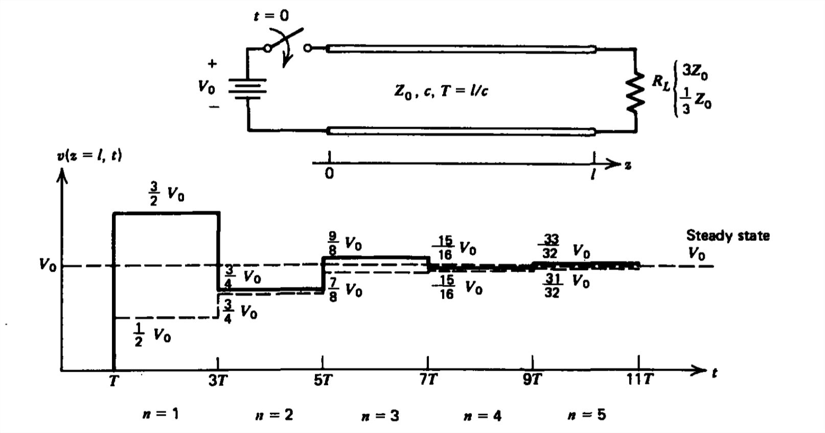
\(\Gamma _{s}\Gamma _{L}=\pm \frac{1}{2}\). Then (26) becomes

\[ \textrm{V}_{n}=\left\{\begin{matrix}
\textrm{V}_{0}\left [ 1-\left ( -\frac{1}{2} \right )^{n} \right ],\quad R_{L}=3Z_{0}\\ 
\textrm{V}_{0}\left [ 1-\left ( \frac{1}{2} \right )^{n} \right ],\quad R_{L}=\frac{1}{3}Z_{0}
\end{matrix}\right. \]

The step changes in load voltage oscillate about the steady-state value \(V_{\infty }=V_{0}\). The steps rapidly become smaller having less than one-percent variation for \(n >7\).

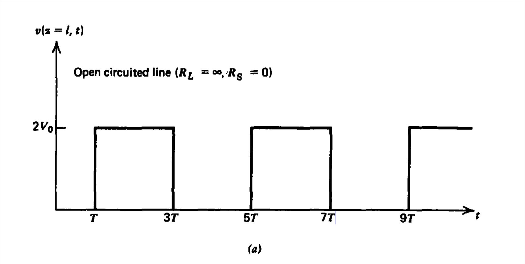
If the source resistance is zero and the load resistance is either zero or infinite (short or open circuits), a lossless transmission line never reiches a dc steady state as the limit of
(27) does not hold with \(\Gamma _{s}\Gamma _{L}=\pm 1\). Continuous reflections with no decrease in amplitude results in pulse waveforms for all time. However, in a real transmission line, small losses in the conductors and dielectric allow a steady state to be eventually reached.

Consider the case when \(R_{s}=0\) and \(R_{L}= \infty \) so that \(\Gamma _{s}\Gamma _{L}=-1\). Then from (26) we have

\[\textrm{V}_{n}=\left\{\begin{matrix}
0,\quad n\,\textrm{even}\\ 
2V_0,\quad n\,\textrm{odd}
\end{matrix}\right. \]

which is sketched in Figure 8-11 a.

For any source and load resistances the current through the load resistor at \(z = l\) is

\begin{align}I_{n}&=\frac{\textrm{V}_{n}}{R_L}=\frac{V_{0}\Gamma _{0}\left ( 1+\Gamma _{L} \right )}{R_L\left ( 1-\Gamma _{s}\Gamma _{L} \right )}\left [1- \left ( \Gamma _{s}\Gamma _{L} \right )^{n} \right ] \\ &
=\frac{2V_{0}\Gamma _{0}}{R_L+Z_0}\frac{1- \left ( \Gamma _{s}\Gamma _{L} \right )^{n}}{\left ( 1-\Gamma _{s}\Gamma _{L} \right )} \nonumber \end{align}

If both \(R_{s}\) and \(R_{L}\) are zero so that \(\Gamma _{s}\Gamma _{L}=-1\), the short circuit current in (31) is in the indeterminate form \(0/0\), which can be evaluated using l'Hôpital's rule:

\[ \begin{align}\lim_{\Gamma _{s}\Gamma _{L}\rightarrow 1}I_{n}&=\frac{2V_{0}\Gamma _{0}}{R_L+Z_0}\frac{\left [ -n\left ( \Gamma _{s}\Gamma _{L} \right )^{n-1} \right ]}{\left ( -1 \right )} \\ &=\frac{2V_{0}n}{Z_0} \nonumber \end{align} \]

As shown by the solid line in Figure 8-11 b, the current continually increases in a stepwise fashion. As \(n\) increases to infinity, the current also becomes infinite, which is expected for a battery connected across a short circuit.

Inductors and Capacitors as Quasi-static Approximations to Transmission Lines

If the transmission line was one meter long with a free space dielectric medium, the round trip transit time \(2 T= 2l/c\)

Figure 8-11 The (a) open circuit voltage and (b) short circuit current at the \(z = l\) end of the transmission line for \(R_{s}=0\). No dc steady state is reached because the system is lossless. If the short circuited transmission line is modeled as an inductor in the quasi-static limit, a step voltage input results in a linearly increasing current (shown dashed). The exact transmission line response is the solid staircase waveform.

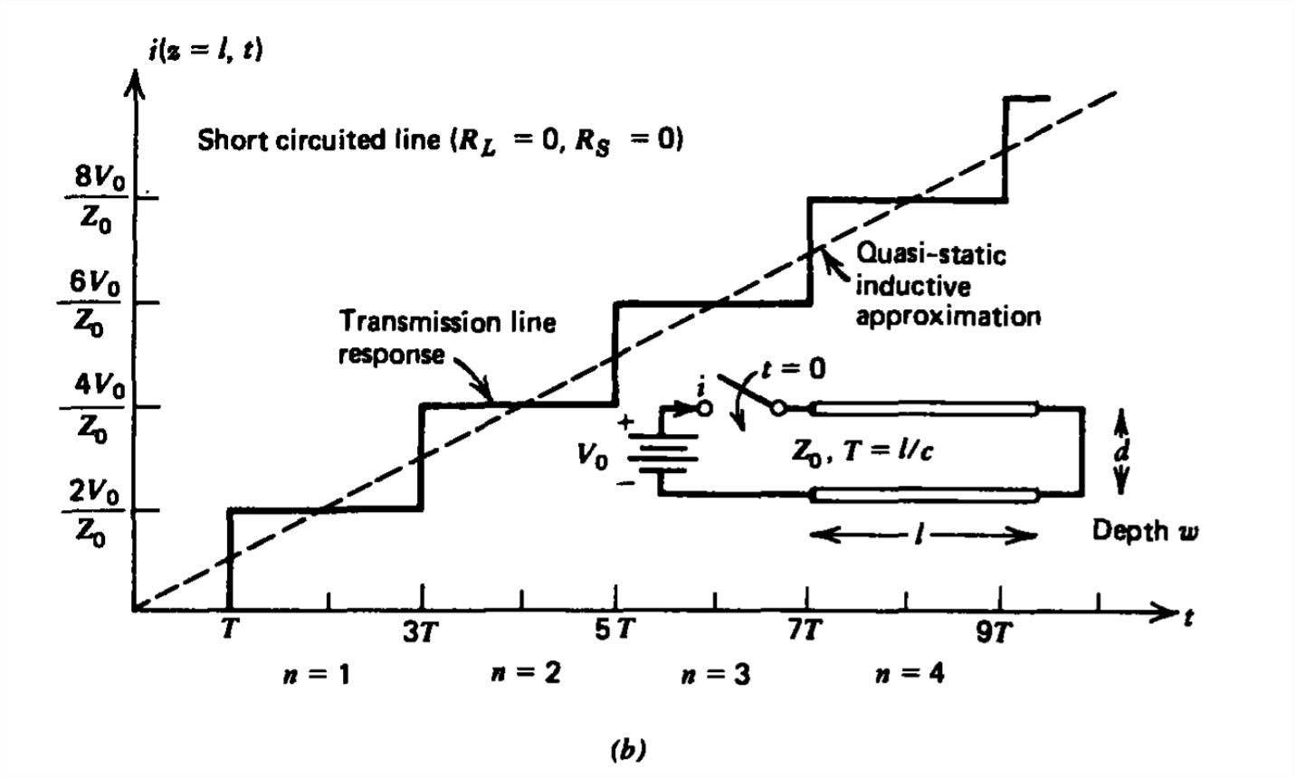
is approximately \(6\) nsec. For many circuit applications this time is so fast that it may be considered instantaneous. In this limit the quasi-static circuit element approximation is valid.

For example, consider again the short circuited transmission line \(\left ( R_{L}=0  \right )\) of length \(l\) with zero source resistance. In the magnetic quasi-static limit we would call the structure an inductor with inductance \(Ll\) (remember, \(L\) is the inductance per unit length) so that the terminal voltage and current are related as

\[ v=\left ( Ll \right )\frac{di}{dt} \]

If a constant voltage \(V_{0}\) is applied at \(t =0\), the current is obtained by integration of (33) as

\[ i=\frac{V_{0}}{Ll}t \]

where we use the initial condition of zero current at \(t = 0\). The linear time dependence of the current, plotted as the dashed line in Figure 8-11 b, approximates the rising staircase waveform obtained from the exact transmission line analysis of (32).

Similarly, if the transmission line were open circuited with \(R_{L}=\infty \), it would be a capacitor of value \(Cl\) in the electric quasi-static limit so that the voltage on the line charges up through the source resistance \(R_{s}\) with time constant \(\tau =R_{s}Cl\) as

\[ v\left ( t \right )=V_{0}\left ( 1-e^{-t/\tau } \right ) \]

The exact transmission line voltage at the \(z = l\) end is given by (26) with \(R_{L}=\infty \) so that \(\Gamma _{L}= 1\):

\[ \textrm{V}_{n}=V_{0}\left ( 1- \Gamma _{s}^{n}\right ) \]

where the source reflection coefficient can be written as

\[ \begin{align}\Gamma _{s}&=\frac{R_{s}-Z_{s}}{R_{s}+Z_{s}} \\ &=\frac{R_{s}-\sqrt{L/C}}{R_{s}+\sqrt{L/C}} \nonumber \end{align} \]

If we multiply the numerator and denominator of (37) through by \(Cl\), we have

\[ \begin{align}\Gamma _{s}&=\frac{R_{s}Cl-l\sqrt{L/C}}{R_{s}Cl+l\sqrt{L/C}} \\ &=\frac{\tau -T}{\tau +T}=\frac{1-T/\tau}{1+T/\tau} \nonumber \end{align} \]

where

\[ T=l\sqrt{L/C}=l/c \]

For the quasi-static limit to be valid, the wave transit time \(T\) must be much faster than any other time scale of interest so that \(T/\tau \ll 1\). In Figure 8-12 we plot (35) and (36) for two values of \(T/\tau\) and see that the quasi-static and transmission line results approach each other as \(T/\tau\) becomes small.

When the roundtrip wave transit time is so small compared to the time scale of interest so as to appear to be instantaneous, the circuit treatment is an excellent approximation.

Figure 8-12 The open circuit voltage at \(z= l\) for a step voltage applied at \(t=0\) through a source resistance \(R_{s}\) for various values of \(T/\tau\), which is the ratio of propagation time \(T= l/c\) to quasi-static charging time \(\tau=R_{s}Cl\). The dashed curve shows the exponential rise obtained by a circuit analysis assuming the open circuited transmission line is a capacitor.

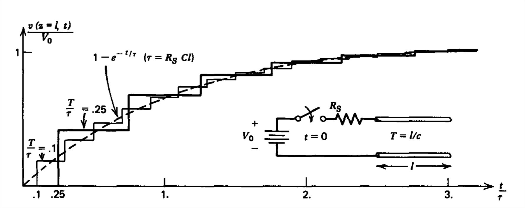
If this propagation time is significant, then the transmission line equations must be used.

Reflections from Arbitrary Terminations

For resistive terminations we have been able to relate reflected wave amplitudes in terms of an incident wave amplitude through the use of a reflection coefficient becauise the voltage and current in the resistor are algebraically related. For an arbitrary termination, which may include any component such as capacitors, inductors, diodes, transistors, or even another transmission line with perhaps a different characteristic impedance, it is necessary to solve a circuit problem at the end of the line. For the arbitrary element with voltage \(V_L\) and current \(I_L\) at \(z = l\), shown in Figure 8-13a, the voltage and current at the end of line are related as

\[ v\left ( z=l,t \right )=V_{L}\left ( t \right )=\textrm{V}_{+}\left ( t-l/c \right )+\textrm{V}_{-}\left ( t+l/c \right )\]
\[i\left ( z=l,t \right )=I_{L}\left ( t \right )=Y_{0}\left [\textrm{V}_{+}\left ( t-l/c \right )-\textrm{V}_{-}\left ( t+l/c \right )  \right ] \]

We assume that we know the incident \(\textrm{V}_{+}\) wave and wish to find the reflected \(\textrm{V}_{-}\) wave. We then eliminate the unknown \(\textrm{V}_{-}\) in (40) and (41) to obtain

\[ 2\textrm{V}_{+}\left ( t-l/c \right )=\textrm{V}_{L}\left ( t \right )+I_{L}\left ( t \right )Z_{0} \]

which suggests the equivalent circuit in Figure 8-13b.

For a particular lumped termination we solve the equivalent circuit for \(\textrm{V}_{L}\left ( t \right )\) or \(I_{L}\left ( t \right )\). Since \(\textrm{V}_{+}\left ( t-l/c \right )\) is already known as it is incident upon the termination, once \(\textrm{V}_{L}\left ( t \right )\) or

Figure 8-13 A transmission line with an (a) arbitrary load at the \(z= l\) end can be analyzed from the equivalent circuit in (b). Since \(\textrm{V}_{+}\) is known, calculation of the load current or voltage yields the reflected wave \(\textrm{V}_{-}\).

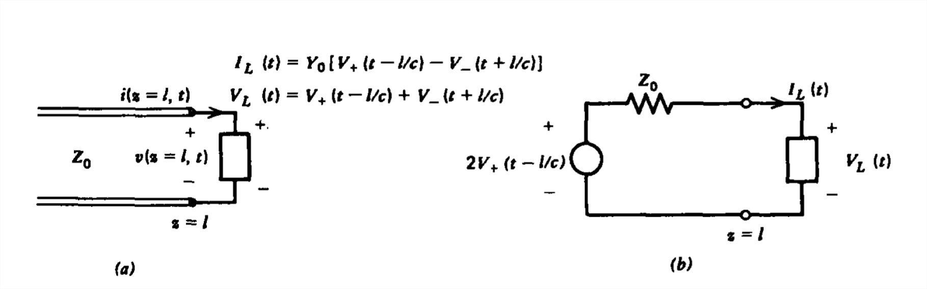
\(I_{L}\left ( t \right )\) is calculated from the equivalent circuit, \(\textrm{V}_{-}\left ( t+l/c \right )\) can be calculated as \(\textrm{V}_{-}=\textrm{V}_{L}-\textrm{V}_{+}\).

For instance, consider the lossless transmission lines of length \(l\) shown in Figure 8-14a terminated at the end with either a lumped capacitor \(C_L\) or an inductor \(L_L\). A step voltage at \(t=0\) is applied at \(z=0\) through a source resistor matched to the line.

The source at z =0 is unaware of the termination at \(z=l\) until a time \(2T\). Until this time it launches a \(\textrm{V}_{+}\) wave of amplitude \(\textrm{V}_{0}/2\). At \(z = l\), the equivalent circuit for the capacitive termination is shown in Figure 8-14b. Whereas resistive terminations just altered wave amplitudes upon reflection, inductive and capacitive terminations introduce differential equations.

From (42), the voltage across the capacitor \(v_c\) obeys the differential equation

\[ Z_{0}C_{L}\frac{dv_{c}}{dt}+v_{c}=2\textrm{V}_{+}=V_{0},\quad t>T \]

with solution

\[v_{c}\left ( t \right )=V_{0}\left [ 1-e^{-\left ( t-T \right )/Z_{0}C_{L}} \right ],\quad t>T \]

Note that the voltage waveform plotted in Figure 8-14b begins at time \(T= l/c\).

Thus, the returning \(\textrm{V}_{-}\) wave is given as

\[ \textrm{V}_{-}=v_{c}-\textrm{V}_{+}=V_0/2+V_0e^{-\left ( t-T \right )/Z_{0}C_{L}} \]

This reflected wave travels back to \(z =0\), where no further reflections occur since the source end is matched. The current at \(z = l\) is then

\[i_{c}=C_{L}\frac{dv_{c}}{dt}=\frac{V_{0}}{Z_{0}}e^{-\left ( t-T \right )/Z_{0}C_{L}},\quad t>T \]

and is also plotted in Figure 8-14b.

Figure 8-14 (a) A step voltage is applied to transmission lines loaded at \(z =l\) with a capacitor \(C_L\) or inductor \(L_L\). The load voltage and current are calculated from the (b) resistive-capacitive or (c) resistive-inductive equivalent circuits at \(z = l\) to yield exponential waveforms with respective time constants \(\tau =Z_{0}C_{L}\) and \(\tau =L_{L}/Z_{0}\) as the solutions approach the dc steady state. The waveforms begin after the initial \(\textrm{V}_{+}\) wave arrives at \(z = l\) after a time \(T=l/c\). There are no further reflections as the source end is matched.

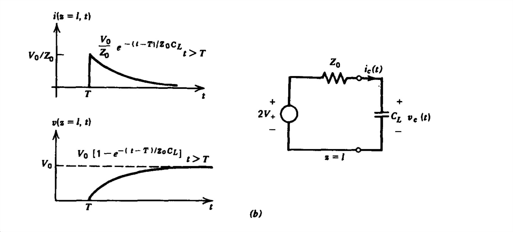
If the end at \(z =0\) were not matched, a new \(\textrm{V}_{+}\) would be generated. When it reached \(z = l\), we would again solve the \(RC\) circuit with the capacitor now initially charged. The reflections would continue, eventually becoming negligible if \(R_{s}\) is nonzero.

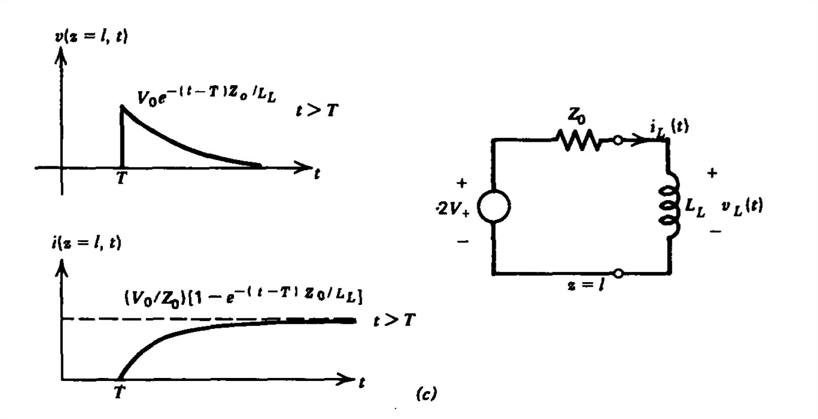
Similarly, the governing differential equation for the inductive load obtained from the equivalent circuit in Figure 8-14c is

\[ L_{L}\frac{di_{L}}{dt}+i_{L}Z_{0}=2\textrm{V}_{+}=V_{0},\quad t>T \]

with solution

\[ i_{L}=\frac{V_{0}}{Z_{0}}\left ( 1-e^{-\left ( t-T \right )Z_{0}/L_{L}} \right ),\quad t>T \]

The voltage across the inductor is

\[ v_{L}=L_{L}\frac{di_{L}}{dt}=V_{0}e^{-\left ( t-T \right )Z_{0}/L_{L}},\quad t>T \]

Again since the end at \(z =0\) is matched, the returning \(\textrm{V}_{-}\) wave from \(z = l\) is not reflected at \(z =0\). Thus the total voltage and current for all time at \(z = l\) is given by (48) and (49) and is sketched in Figure 8-14c.