8.3: Sinusoidal Time Variations

Solutions to the Transmission Line Equations

Often transmission lines are excited by sinusoidally varying sources so that the line voltage and current also vary sinusoidally with time:

\[ v\left ( z,t \right )=\textrm{Re}\left [ \hat{v}\left ( z \right )e^{j\omega t} \right ]\\
i\left ( z,t \right )=\textrm{Re}\left [ \hat{i}\left ( z \right )e^{j\omega t} \right ] \]

Then as we found for TEM waves in Section 7-4, the voltage and current are found from the wave equation solutions of Section 8-1-5 as linear combinations of exponential functions with arguments \(t-z/c\) and \(t+z/c\):

\[ v\left ( z,t \right )=\textrm{Re}\left [ \hat{\textrm{V}}_{+}e^{j\omega \left ( t-z/c \right )}+\hat{\textrm{V}}_{-}e^{j\omega \left ( t+z/c \right )} \right ]\\
i\left ( z,t \right )=Y_{0}\textrm{Re}\left [ \hat{\textrm{V}}_{+}e^{j\omega \left ( t-z/c \right )}-\hat{\textrm{V}}_{-}e^{j\omega \left ( t+z/c \right )} \right ] \]

Now the phasor amplitudes \(\hat{\textrm{V}}_{+}\) and \(\hat{\textrm{V}}_{-}\) are complex numbers and do not depend on \(z\) or \(t\).

By factoring out the sinusoidal time dependence in (2), the spatial dependences of the voltage and current are

\[ \hat{v}\left ( z \right )=\hat{\textrm{V}}_{+}e^{-jkz}+\hat{\textrm{V}}_{-}e^{+jkz}\\
\hat{i}\left ( z \right )=Y_{0}\left (  \hat{\textrm{V}}_{+}e^{-jkz}-\hat{\textrm{V}}_{-}e^{+jkz}\right ) \]

where the wavenumber is again defined as

\[ k=\omega /c \]

Lossless Terminations

(a) Short Circuited Line

The transmission line shown in Figure 8-15a is excited by a sinusoidal voltage source at \(z = -l\) imposing the boundary condition

\[ \begin{align} v\left ( z=-l,t \right )&=V_{0}\cos \omega t \\ &
=\textrm{Re}\left ( V_{0}e^{j\omega t} \right )\Rightarrow \hat{v}\left ( z=-l \right )=V_{0}=\hat{\textrm{V}}_{+}e^{jkl}+\hat{\textrm{V}}_{-}e^{-jkl} \nonumber \end{align} \]

Note that to use (3) we must write all sinusoids in complex notation. Then since all time variations are of the form \(e^{j\omega t}\), we may suppress writing it each time and work only with the spatial variations of (3).

Because the transmission line is short circuited, we have the additional boundary condition

\[ v\left ( z=0,t \right )=0\Rightarrow \hat{v}\left ( z=0 \right )=0=\hat{\textrm{V}}_{+}+\hat{\textrm{V}}_{-} \]

which when simultaneously solved with (5) yields

\[ \hat{\textrm{V}}_{+}=-\hat{\textrm{V}}_{-}=\frac{V_{0}}{2j\sin kl} \]

The spatial dependences of the voltage and current are then

\[ \hat{v}\left ( z\right )=\frac{V_{0}\left ( e^{-jkz}-e^{jkz} \right )}{2j\sin kl}=-\frac{V_{0}\sin kz}{\sin kl}\\
\hat{i}\left ( z\right )=\frac{V_{0}Y_{0}\left ( e^{-jkz}+e^{+jkz} \right )}{2j\sin kl}=-j\frac{V_{0}Y_{0}\cos kz}{\sin kl} \]

The instantaneous voltage and current as functions of space and time are then

\[ v\left ( z,t \right )=\textrm{Re}\left [ \hat{v}\left ( z\right )e^{j\omega t} \right ]=-V_{0}\frac{\sin kz}{\sin kl}\cos \omega t\\
i\left ( z,t \right )=\textrm{Re}\left [ \hat{i}\left ( z\right )e^{j\omega t} \right ]=\frac{V_{0}Y_{0}\cos kz\sin \omega z}{\sin kl} \]

Figure 8-15 The voltage and current distributions on a (a) short circuited and (b) open circuited transmission line excited by sinusoidal voltage sources at \(z = -l\) If the lines are much shorter than a wavelength, they act like reactive circuit elements. (c) As the frequency is raised, the impedance reflected back as a function of \(\)z can look capacitive or inductive making the transition through open or short circuits.

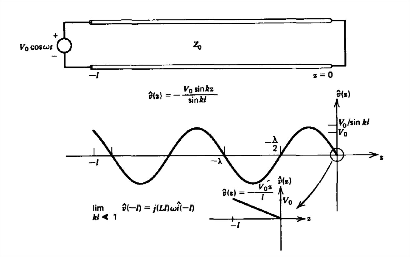
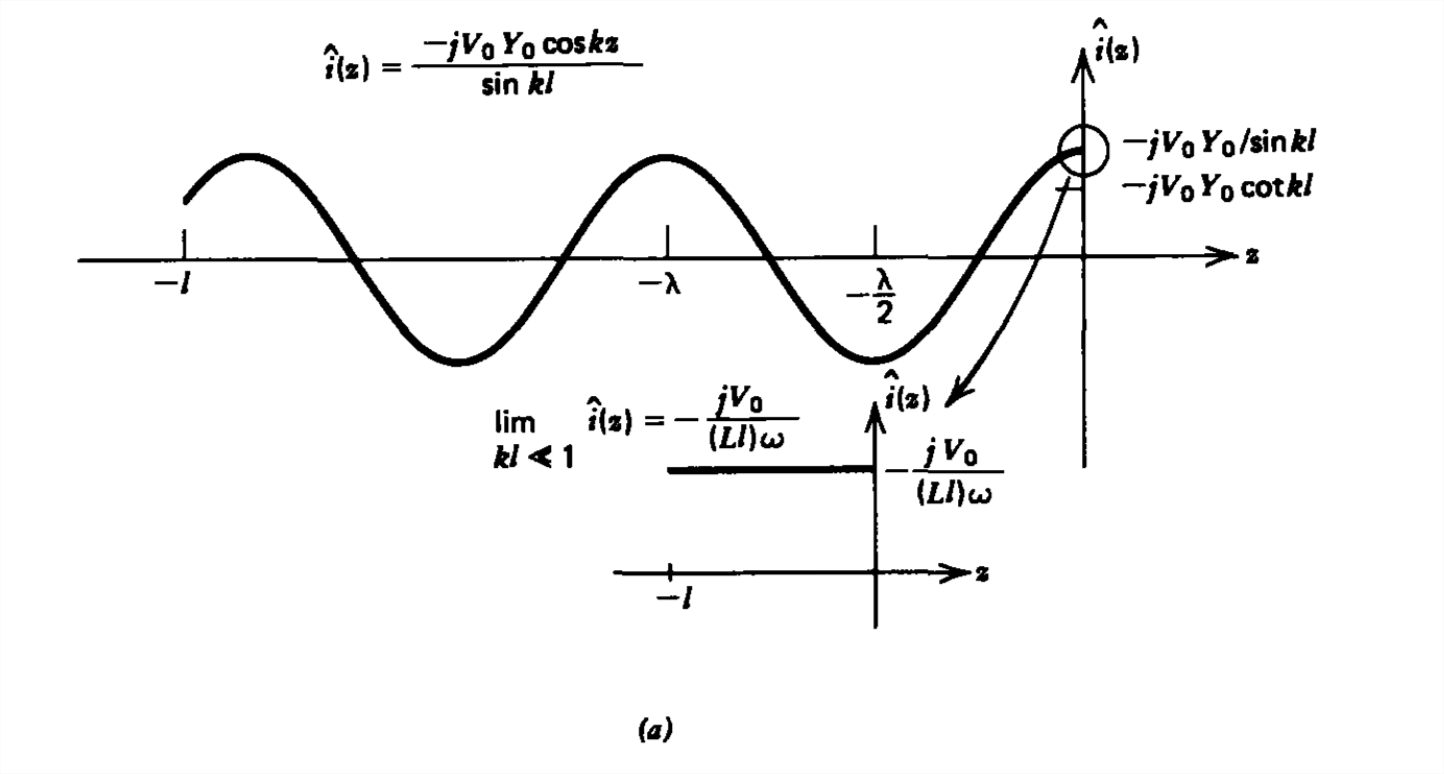
The spatial distributions of voltage and current as a function of \(z\) at a specific instant of time are plotted in Figure 8-15a and are seen to be \(90^{\circ }\) out of phase with one another in space with their distributions periodic with wavelength \(\lambda \) given by

\[ \lambda =\frac{2\pi }{k}=\frac{2\pi c}{\omega } \]

The complex impedance at any position \(z\) is defined as

\[ Z\left ( z \right )=\frac{\hat{v}\left ( z\right )}{\hat{i}\left ( z\right )} \]

which for this special case of a short circuited line is found from (8) as

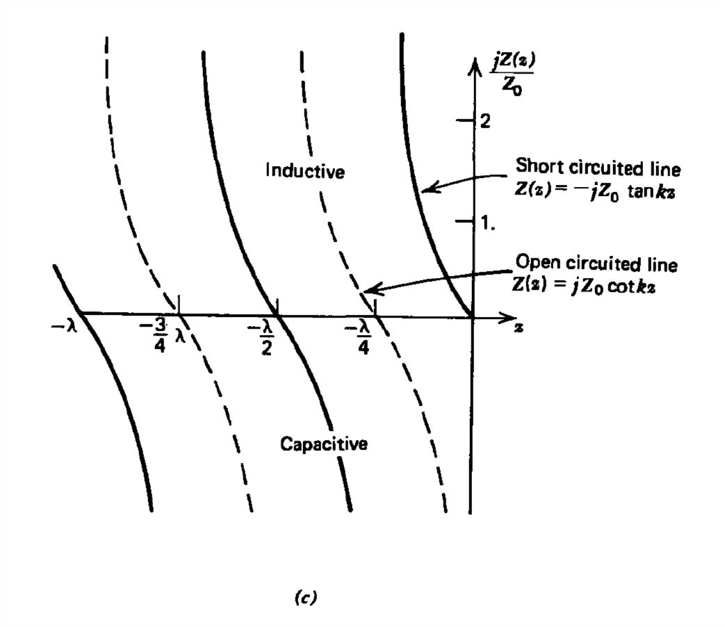
\[ Z\left ( z \right )=-jZ_{0}\tan kz \]

In particular, at \(z= -l\), the transmission line appears to the generator as an impedance of value

\[ Z\left ( z=-l \right )=jZ_{0}\tan kz \]

From the solid lines in Figure 8-15c we see that there are various regimes of interest:

1. When the line is an integer multiple of a half wavelength long so that \(kl=n\pi ,\,n=1,2,3,...\), the impedance at \(z= -l\) is zero and the transmission line looks like a short circuit.
2. When the-line is an odd integer multiple of a quarter wavelength long so that \(kl=\left ( 2n-1 \right )\pi/2 ,\,n=1,2,...\), the impedance at \(z = -l\) is infinite and the transmission line looks like an open circuit.
3. Between the short and open circuit limits \(\left ( n-1 \right )\pi < kl< \left ( 2n-1 \right )\pi/2,\,n=1,2,3,...\), \(Z\left ( z=-l \right )\) has a positive reactance and hence looks like an inductor.
4. Between the open and short circuit limits \(\left ( n-\frac{1}{2} \right )\pi < kl< n\pi/2,\,n=1,2,...\), \(Z\left ( z=-l \right )\) has a negative reactance arid so looks like a capacitor.

Thus, the short circuited transmission line takes on all reactive values, both positive (inductive) and negative (capacitive), including open and short circuits as a function of \(kl\) Thus, if either the length of the line \(l\) or the frequency is changed, the impedance of the transmission line is changed.

Examining (8) we also notice that if \(\sin kl=0,\,\left ( kl=n\pi ,\,n=1,2,... \right )\), the voltage and current become infinite (in practice the voltage and current become large limited only by losses). Under these conditions, the system is said to be resonant with the resonant frequencies given by

\[ \omega _{n}=n\pi c/l,\quad n=1,2,3,... \]

Any voltage source applied at these frequencies will result in very large voltages and currents on the line.

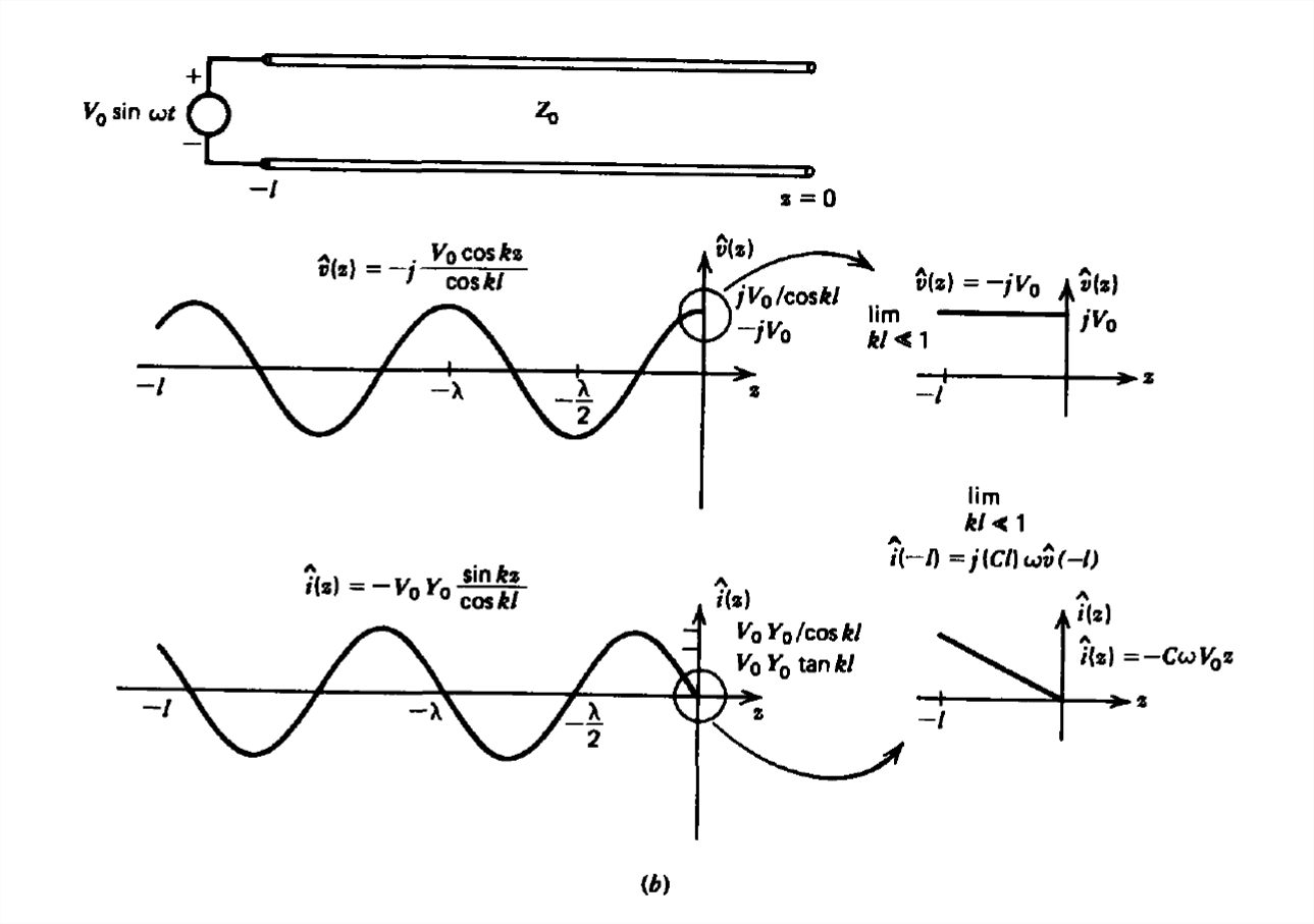
(b) Open Circuited Line

If the short circuit is replaced by an open circuit, as in Figure 8-15b, and for variety we change the source at \(z = -l\) to \(V_{0}\sin \omega t\) the boundary conditions are

\[ i\left ( z=0,t \right )=0\\
v\left ( z=-l,t \right )=V_{0}\sin \omega t=\textrm{Re}\left ( -jV_{0}e^{j\omega t} \right ) \]

Using (3) the complex amplitudes obey the relations

\[ \hat{i}\left ( z=0 \right )=0=Y_{0}\left (\textrm{V}_{+}-\textrm{V}_{-}  \right )\\
\hat{v}\left ( z=-l\right )=-jV_{0}=\textrm{V}_{+}e^{jkl}+\textrm{V}_{-}e^{-jkl} \]

which has solutions

\[ \hat{\textrm{V}}_{+}=\hat{\textrm{V}}_{-}=\frac{-jV_{0}}{2\cos kl} \]

The spatial dependences of the voltage and current are then

\[ \hat{v}\left ( z \right )=\frac{-jV_{0}}{2\cos kl}\left ( e^{-jkz}+e^{jkz} \right )=\frac{-jV_{0}}{\cos kl}\cos kz\\
\hat{\imath }\left ( z \right )=\frac{-jV_{0}Y_{0}}{2\cos kl}\left ( e^{-jkz}-e^{+jkz} \right )=-\frac{V_{0}Y_{0}}{\cos kl}\sin kz  \]

with instantaneous solutions as a function of space and time: 

\[ v\left ( z,t \right )=\textrm{Re}\left [ \hat{v}\left ( z \right )e^{j\omega t} \right ]=\frac{V_{0}\cos kz}{\cos kl}\sin \omega t\\
i\left ( z,t \right )=\textrm{Re}\left [ \hat{\imath }\left ( z \right )e^{j\omega t} \right ]=-\frac{V_{0}Y_{0}}{\cos kl}\sin kz\cos \omega t \]

The impedance at \(z = -l\) is

\[ Z\left ( z=-l \right )=\frac{\hat{v}\left ( -l \right )}{\hat{\imath }\left ( -l \right )}=-jZ_{0}\cot kl \]

Again the impedance is purely reactive, as shown by the dashed lines in Figure 8-15c, alternating signs every quarter wavelength so that the open circuit load looks to the voltage source as an inductor, capacitor, short or open circuit depending on the frequency and length of the line.

Resonance will occur if

\[ \cos kl=0 \]

or

\[ kl=\left ( 2n-1 \right )\pi /2,\quad n=1,2,3,... \]

so that the resonant frequencies are

\[ \omega _{n}=\frac{\left ( 2n-1 \right )\pi c}{2l} \]

Reactive Circuit Elements as Approximations to Short Transmission Lines

Let us re-examine the results obtained for short and open circuited lines in the limit when \(l\) is much shorter than the wavelength \(\lambda \) so that in this long wavelength limit the spatial trigonometric functions can be approximated as

\[ \lim_{kl\ll 1}\left\{\begin{matrix}
\sin kz\approx kz\\ 
\cos kz\approx 1
\end{matrix}\right. \]

Using these approximations, the voltage, current, and impedance for the short circuited line excited by a voltage source \(V_{0}\cos \omega t\) can be obtained from (9) and (13) as

\begin{align} \lim_{kl\ll 1}\left\{\begin{array}{lr} 
v\left ( z,t \right )=\frac{V_{0}z}{l}\cos \omega t,\quad v\left ( -l,t \right )=V_{0}\cos \omega t &\\
i\left ( z,t \right )=\frac{V_{0}Y_{0}}{kl}\sin \omega t,\quad i\left ( -l,t \right )=\frac{V_{0}\sin \omega t}{\left ( Ll \right )\omega }&\\
Z\left ( -l \right )=jZ_{0}kl=j\frac{\omega Z_{0}l}{c}=j\omega \left ( Ll \right )&
\end{array}\right.\end{align}

We see that the short circuited transmission line acts as an inductor of value \(\left ( Ll \right )\) (remember that \(L\) is the inductance per unit length), where we used the relations

\[ Z_{0}=\frac{1}{Y_{0}}=\sqrt{\frac{L}{C}},\quad c=\frac{1}{\sqrt{LC}} \]

Note that at \( z=-l\),

\[ v\left ( -l,t \right )=\left ( Ll \right )\frac{di\left ( -l,t \right )}{dt} \]

Similarly for the open circuited line we obtain:

\begin{align}\lim_{kl\ll 1}\left\{
\begin{array}{lr}
v\left ( z,t \right )=V_{0}\sin \omega t&\\ 
i\left ( z,t \right )=-V_{0}Y_{0}kz\cos \omega t&\\ 
Z\left ( -l \right )=\frac{-jZ_{0}}{kl}=\frac{-j}{\left ( Cl \right )\omega }&
\end{array}\right.\quad i\left ( -l,t \right )=\left ( Cl \right )\omega V_{0}\cos \omega t  
\end{align}  

For the open circuited transmission line, the terminal voltage and current are simply related as for a capacitor,

\[ i\left ( -l,t \right )=\left ( Cl \right )\frac{dv\left ( -l,t \right )}{dt} \]

with capacitance given by \(\left ( Cl \right )\).

In general, if the frequency of excitation is low enough so that the length of a transmission line is much shorter than the wavelength, the circuit approximations of inductance and capacitance are appropriate. However, it must be remembered that if the frequencies of interest are so high that the length of a circuit element is comparable to the wavelength, it no longer acts like that element. In fact, as found in Section 8-3-2, a capacitor can even look like an inductor, a short circuit, or an open circuit at high enough frequency while vice versa an inductor can also look capacitive, a short or an open circuit.

In general, if the termination is neither a short nor an open circuit, the voltage and current distribution becomes more involved to calculate and is the subject of Section 8-4.

Effects of Line Losses

(a) Distributed Circuit Approach

If the dielectric and transmission line walls have Ohmic losses, the voltage and current waves decay as they propagate. Because the governing equations of Section 8-1-3 are linear with constant coefficients, in the sinusoidal steady state we assume solutions of the form

\[ v\left ( z,t \right )=\textrm{Re}\left ( \hat{V}e^{j\left ( \omega t-kz \right )} \right )\\
i\left ( z,t \right )=\textrm{Re}\left ( \hat{I}e^{j\left ( \omega t-kz \right )} \right ) \]

where now \(\omega \) and \(k\) are not simply related as the nondispersive relation in (4). Rather we substitute (30) into Eq. (28) in Section 8-1-3:

\[ \frac{\partial i}{\partial z}=-C\frac{\partial v}{\partial t}-Gv\Rightarrow -jk\hat{I}=-\left ( Cj\omega +G \right )\hat{V}\\
\frac{\partial v}{\partial z}=-L\frac{\partial i}{\partial t}-iR\Rightarrow -jk\hat{V}=-\left ( Lj\omega +R \right )\hat{I} \]

which requires that

\[ \frac{\hat{V}}{\hat{I}}=\frac{jk}{\left ( Cj\omega +G \right )}=\frac{Lj\omega +R}{jk} \]

We solve (32) self-consistently for \(k\) as

\[ k^{2}=-\left ( Lj\omega +R \right )\left ( Cj\omega +G \right )=LC\omega ^{2}-j\omega \left ( RC+LG \right )-RG \]

The wavenumber is thus complex so that we find the real and imaginary parts from (33) as

\begin{align} k=k_{r}+jk_{i}\Rightarrow k_{r}^{2}-k_{i}^{2}&=LC\omega ^{2}-RG \\
2k_{r}k_{i}&=-\omega \left ( RC+LG \right ) \nonumber \end{align}

In the low loss limit where \(\omega RC\ll 1\) and \(\omega LG\ll 1\), the spatial decay of \(k_i\) is small compared to the propagation wavenumber \(k_r\). In this limit we have the following approximate solution:

\begin{align} 
\lim_{\omega RC\ll 1\\\omega LG\ll 1}\left\{\begin{array}
k_{r}\approx \pm \omega \sqrt{LC}\pm \omega /c&\\ 
k_{i}=-\frac{\omega \left ( RC+LG \right )}{2k_{r}}&\approx \mp \frac{1}{2}\left [ R\sqrt{\frac{C}{L}}+G\sqrt{\frac{L}{C}} \right ]\\ 
& \approx \mp \frac{1}{2}\left ( RY_{0}+GZ_{0} \right )
\end{array}\right.  \end{align}

We use the upper sign for waves propagating in the \(+z\) direction and the lower sign for waves traveling in the \(-z\) direction.

(b) Distortionless lines

Using the value of \(k\) of (33),

\[ k=\pm \left [ -\left ( Lj\omega +R \right )\left ( Cj\omega +G \right ) \right ]^{2} \]

in (32) gives us the frequency dependent wave impedance for waves traveling in the \(\pm z\) direction as

\[ \frac{\hat{V}}{\hat{I}}=\pm \left ( \frac{Lj\omega +R }{Cj\omega +G} \right )^{1/2}=\pm \sqrt{\frac{L}{C}}\left ( \frac{j\omega +R/L}{j\omega +G/C} \right )^{1/2} \]

If the line parameters are adjusted so that

\[ \frac{R}{L}=\frac{G}{C} \]

the impedance in (37) becomes frequency independent and equal to the lossless line impedance. Under the conditions of (38) the complex wavenumber reduces to

\[ k_{r}=\pm \omega \sqrt{LC},\quad k_{i}=\mp \sqrt{RG} \]

Although the waves are attenuated, all frequencies propagate at the same phase and group velocities as for a lossless line

\[ v_{p}=\frac{\omega }{k_{r}}=\pm \frac{1}{\sqrt{LC}}\\
v_{g}=\frac{d\omega }{dk_{r}}=\pm \frac{1}{\sqrt{LC}} \]

Since all the Fourier components of a pulse excitation will travel at the same speed, the shape of the pulse remains unchanged as it propagates down the line. Such lines are called distortionless.

(c) Fields Approach

If \(R = 0\), we can directly find the TEM wave solutions using the same solutions found for plane waves in Section 7-4-3. There we found that a dielectric with permittivity \(\varepsilon\)  and small Ohmic conductivity \(\sigma \) has a complex wavenumber:

\[ \lim_{\sigma /\omega \varepsilon \ll 1}k\approx \left ( \frac{\omega }{c}-\frac{j\sigma \eta }{2} \right ) \]

Equating (41) to (35) with \(R =0\) requires that \(GZ_{0}=\sigma \eta \).

The tangential component of \(\textbf{H}\) at the perfectly conducting transmission line walls is discontinuous by a surface current. However, if the wall has a large but noninfinite Ohmic conductivity \(\sigma _{w}\), the fields penetrate in with a characteristic distance equal to the skin depth \(\delta =\sqrt{2/\omega \mu \sigma _{w}}\). The resulting \(z\)-directed current gives rise to a \(z\)-directed electric field so that the waves are no longer purely TEM.

Because we assume this loss to be small, we can use an approximate perturbation method to find the spatial decay rate of the fields. We assume that the fields between parallel plane electrodes are essentially the same as when the system is lossless except now being exponentially attenuated as \(e^{-\alpha z}\), where \(\alpha =-k_{i}\):

\[ \begin{align}E_{x}\left ( z,t \right )&=\textrm{Re}\left [ \hat{E}e^{j\left ( \omega t-k_{r}z \right )}e^{-\alpha z} \right ] \\
H_{y}\left ( z,t \right )&=\textrm{Re}\left [ \frac{\hat{E}}{\eta }e^{j\left ( \omega t-k_{r}z \right )}e^{-\alpha z} \right ],\quad k_r=\frac{\omega }{c} \nonumber \end{align} \]

From the real part of the complex Poynting's theorem derived in Section 7-2-4, we relate the divergence of the time-average electromagnetic power density to the time-average dissipated power:

\[ \nabla \cdot <\textbf{S}>=-<P_{d}> \]

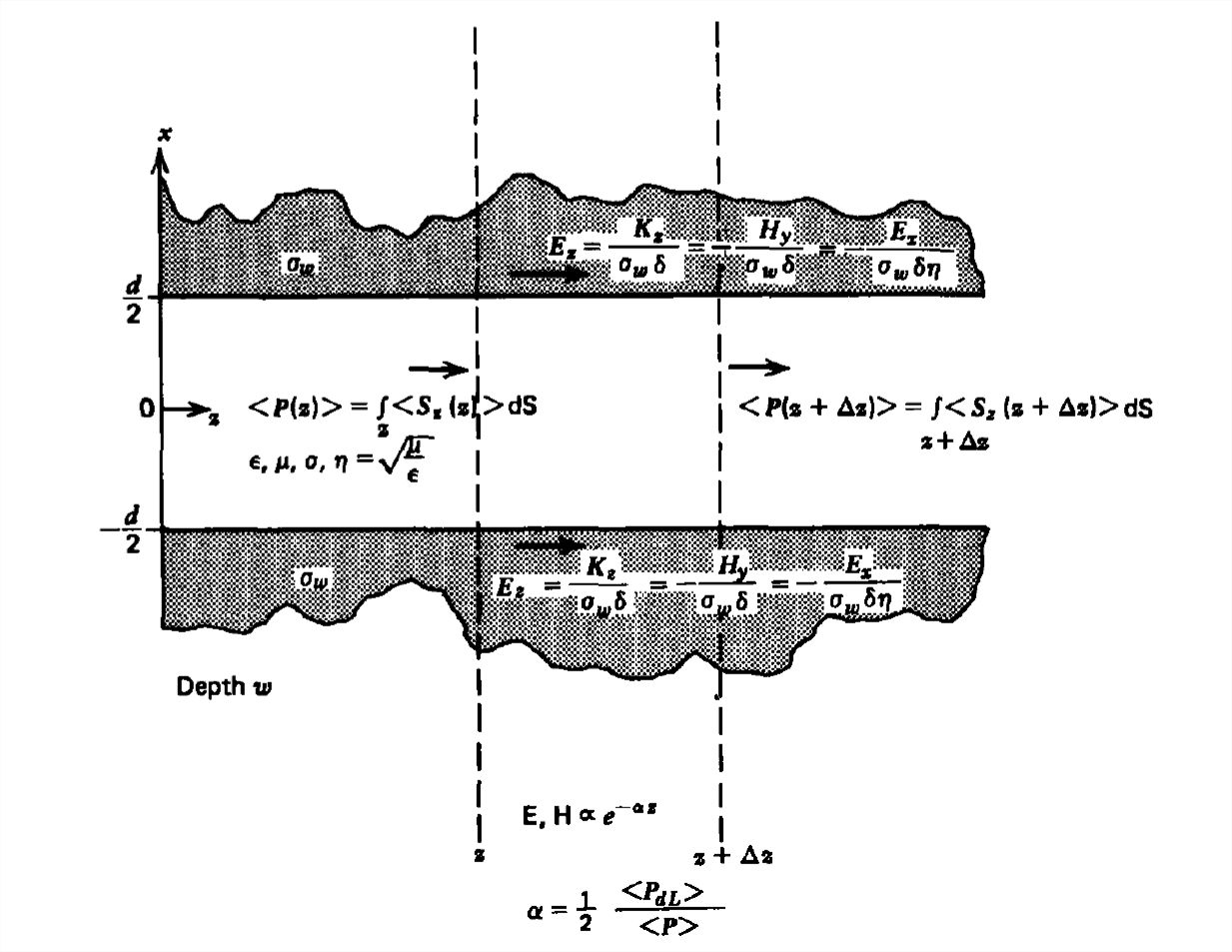
Using the divergence theorem we integrate (43) over a volume of thickness \(\Delta z\) that encompasses the entire width and thickness of the line, as shown in Figure 8-16:

\[ \begin{align}\int_{\textrm{V}}\nabla \cdot <\textbf{S}>d\textrm{V}&=\oint_{\textrm{S}} <\textbf{S}>\cdot \textbf{dS} \\
&=\int_{z+\Delta z}<S_{z}\left ( z+\Delta z\right )>d\textrm{S} \nonumber \\
&\quad-\int_{z}<S_{z}\left ( z\right )>d\textrm{S}=-\int_{\textrm{V}}<P_d>d\textrm{V} \nonumber \end{align} \]

The power \(<P_d>\) is dissipated in the dielectric and in the walls. Defining the total electromagnetic power as

\[ <P(z)>=\int_{z}<S_{z}\left ( z\right )>d\textrm{S} \]

Figure 8-16 A transmission line with lossy walls and dielectric results in waves that decay as they propagate. The spatial decay rate \(\alpha \) of the fields is approximately proportional to the ratio of time average dissipated power per unit length \(<P_{dL}>\) to the total time average electromagnetic power flow \(<P>\) down the line.

(44) can be rewritten as

\[  <P(z+\Delta z)>- <P(z)>=-\int<P_{(d)}>dx\,dy\,dz \]

Dividing through by \(dz = \Delta z\), we have in the infinitesimal limit

\[ \begin{align}\lim_{\Delta z\rightarrow 0}\frac{<P(z+\Delta z)>-<P(z)>}{\Delta z}&=\frac{d<P(z)>}{dz}=-\int_{\textrm{S}}<P_{d}>dx\,dy \\
&=-<P_{dL}> \nonumber \end{align} \]

where \(<P_{dL}>\) is the power dissipated per unit length. Since the fields vary as \(e^{-\alpha z}\), the power flow that is proportional to the square of the fields must vary as \(e^{-2\alpha z}\) so that

\[ \frac{d<P>}{dz}=-2\alpha <P>=-<P_{dL}> \]

which when solved for the spatial decay rate is proportional to the ratio of dissipated power per unit length to the total electromagnetic power flowing down the transmission line:

\[ \alpha =\frac{1}{2}\frac{<P_{dL}>}{<P>} \]

For our lossy transmission line, the power is dissipated both in the walls and in the dielectric. Fortunately, it is not necessary to solve the complicated field problem within the walls because we already approximately know the magnetic field at the walls from (42). Since the wall current is effectively confined to the skin depth \(\delta \), the cross-sectional area through which the current flows is essentially \(w\delta \) so that we can define the surface conductivity as \(\sigma_{w}\delta \), where the electric field at the wall is related to the lossless surface current as

\[ \textbf{K}_{w}=\sigma _{w}\delta \textbf{E}_{w} \]

The surface current in the wall is approximately found from the magnetic field in (42) as

\[ K_{z}=-H_{y}=-E_{x}/\eta  \]

The time-average power dissipated in the wall is then

\[ <P_{dL}>_{\textrm{wall}}=\frac{w}{2}\textrm{Re}\left ( \textbf{E}_{w}\cdot \textbf{K}_{w}^{\ast } \right )=\frac{1}{2}\frac{\left | \textbf{K}_{w} \right |^{2}w}{\sigma _{w}\delta }=\frac{1}{2}\frac{\left | \hat{E} \right |^{2}w}{\sigma _{w}\delta \eta ^{2}} \]

The total time-average dissipated power in the walls and dielectric per unit length for a transmission line system of depth \(w\) and plate spacing \(d\) is then

\[ \begin{align}<P_{dL}>&=2<P_{dL}>_{\textrm{wall}}+\frac{1}{2}\sigma \left | \hat{E} \right |^{2}wd \\&
=\frac{1}{2}\left | \hat{E} \right |^{2}w\left ( \frac{2}{\eta ^{2}\sigma _{w}\delta }+\sigma d \right ) \nonumber \end{align} \]

where we multiply (52) by two because of the losses in both electrodes. The time-average electromagnetic power is

\[ <P>=\frac{1}{2}\frac{\left | \hat{E} \right |^{2}}{\eta }wd \]

so that the spatial decay rate is found from (49) as

\[ \alpha =-k_{i}=\frac{1}{2}\left ( \frac{2}{\eta ^{2}\sigma _{w}\delta }+\sigma d \right )\frac{\eta }{d}=\frac{1}{2}\left ( \sigma \eta +\frac{2}{\eta \sigma _{w}\delta d}\right ) \]

Comparing (55) to (35) we see that

\[ GZ_{0}=\sigma \eta,\quad RY_{0}=\frac{2}{\eta \sigma _{w}\delta d}\\
\Rightarrow Z_{0}=\frac{1}{Y_{0}}=\frac{d}{w}\eta ,\quad G=\frac{\sigma w}{d},\quad R=\frac{2}{\sigma _{w}w\delta } \]