8.5: Stub Tuning

In practice, most sources are connected to a transmission line through a series resistance matched to the line. This eliminates transient reflections when the excitation is turned on or off. To maximize the power flow to a load, it is also necessary for the load impedance reflected back to the source to be equal to the source impedance and thus equal to the characteristic impedance of the line, $Z_{0}$. This matching of the load to the line for an arbitrary termination can only be performed by adding additional elements along the line.

Usually these elements are short circuited transmission lines, called stubs, whose lengths can be varied. The reactance of the stub can be changed over the range from $-j\infty$ to $j\infty$ simply by varying its length, as found in Section 8-3-2, for the short circuited line. Because stubs are usually connected in parallel to a transmission line, it is more convenient to work with admittances rather than impedances as admittances in parallel simply add.

Use of the Smith Chart for Admittance Calculations

Fortunately the Smith chart can also be directly used for admittance calculations where the normalized admittance is defined as

$$Y_{n}\left ( z \right )=\frac{Y\left ( z \right )}{Y_{0}}=\frac{1}{Z_{n}\left ( z \right )}$$

If the normalized load admittance $Y_{nL}$ is known, straightforward impedance calculations first require the computation

$$Z_{nL}=1/Y_{nL}$$

so that we could enter the Smith chart at $Z_{nL}$. Then we rotate by the required angle corresponding to $2kz$ and read the new $Z_{n}\left ( z \right )$. Then we again compute its reciprocal to find

$$Y_{n}\left ( z \right )=1/Z_{n}\left ( z \right )$$

The two operations of taking the reciprocal are tedious. We can use the Smith chart itself to invert the impedance by using the fact that the normalized impedance is inverted by a $\lambda /4$ section of line, so that a rotation of $\Gamma \left ( z \right )$ by $180^{\circ }$ changes a normalized impedance into its reciprocal. Hence, if the admittance is given, we enter the Smith chart with a given value of normalized admittance $Y_{n}$ and rotate by $180^{\circ }$ to find $Z_{n}$. We then rotate by the appropriate number of wavelengths to find $Z_{n}\left ( z \right )$. Finally, we again rotate by $180^{\circ }$ to find $Y_{n}\left ( z \right )=1/Z_{n}\left ( z \right )$. We have actually rotated the reflection coefficient by an angle of $2\pi +2kz$. Rotation by $2\pi$ on the Smith chart, however, brings us back to wherever we started, so that only the $2kz$ rotation is significant. As long as we do an even number of $\pi$ rotations by entering the Smith chart with an admittance and leaving again with an admittance, we can use the Smith chart with normalized admittances exactly as if they were normalized impedances.

Example $\PageIndex{1}$: USE OF THE SMITH CHART FOR ADMITTANCE CALCULATIONS

The load impedance on a $50$-$\textrm{Ohm}$ line is

$$Z_{L}=50\left ( 1+j \right ) \nonumber$$

What is the admittance of the load?

SOLUTION

By direct computation we have

$$Y_{L}=\frac{1}{Z_{L}}=\frac{1}{50\left ( 1+j \right )}=\frac{\left ( 1-j \right )}{100} \nonumber$$

To use the Smith chart we find the normalized impedance at $A$ in Figure 8-23:

$$Z_{nL}=1+j \nonumber$$

Figure 8-23 The Smith chart offers a convenient way to find the reciprocal of a complex number using the property that the normalized impedance reflected back by a quarter wavelength inverts. Thus, the normalized admittance is found by locating the normalized impedance and rotating this point by $180^{\circ }$ about the constant $\left | \Gamma _{L} \right |$ circle.

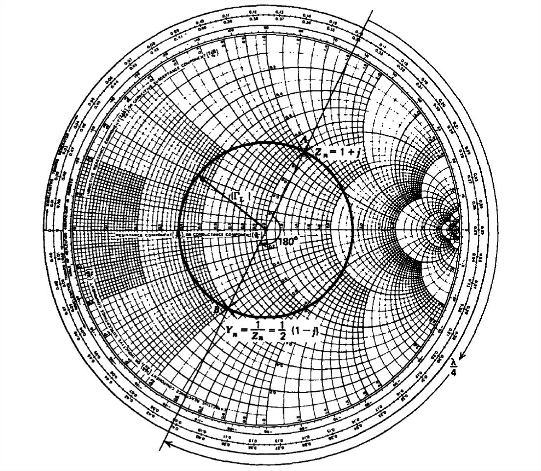
The normalized admittance that is the reciprocal of the normalized impedance is found by locating the impedance a distance $\lambda /4$ away from the load end at $B$:

$$Y_{nL}=0.5\left ( 1-j \right )\Rightarrow Y_{L}=Y_{n}Y_{0}=\left ( 1-j \right )/100 \nonumber$$

Note that the point $B$ is just $180^{\circ }$ away from $A$ on the constant $\left | \Gamma _{L} \right |$ circle. For more complicated loads the Smith chart is a convenient way to find the reciprocal of a complex number.

Single-Stub Matching

A termination of value $Z_{L}=50\left ( 1+j \right )$ on a $50$-$\textrm{Ohm}$ transmission line is to be matched by means of a short circuited stub at a distance L from the load, as shown in Figure 8-24a. We need to find the line length $l_{1}$ and the length of the stub $l_{2}$ such that the impedance at the junction is matched to the line $\left ( Z_{in}=50\,\textrm{Ohm} \right )$. Then we know that all further points to the left of the junction have the same impedance of $50\,\textrm{Ohms}$.

Because of the parallel connection, it is simpler to use the Smith chart as an admittance transformation. The normalized load admittance can be computed using the Smith chart by rotating by $180^{\circ }$ from the normalized load impedance at $A$, as was shown in Figure 8-23 and Example 8-3,

$$Z_{nL}=1+j$$

to yield

$$Y_{nL}=0.5\left ( 1-j \right )$$

at the point $B$.

Now we know from Section 8-3-2 that the short circuited stub can only add an imaginary component to the admittance. Since we want the total normalized admittance to be unity to the left of the stub in Figure 8-24

$$Y_{in}=Y_{1}+Y_{2}=1$$

when $Y_{nL}$ is reflected back to be $Y_{1}$ it must wind up on the circle whose real part is $1$ (as $Y_{2}$ can only be imaginary), which occurs either at $C$ or back at $A$ allowing $l_{1}$ to be either $0.25\lambda$ at $A$ or $\left (0.25 +0.177  \right )\lambda =0.427\lambda$ at $C$ (or these values plus any integer multiple of $\lambda /2$). Then $Y_{1}$ is either of the following two conjugate values:

$$Y_{1}=\left\{\begin{matrix} 1+j,\quad l_{1}=0.25\lambda \,\left ( A \right )\\  1-j,\quad l_{1}=0.427\lambda \,\left ( C \right ) \end{matrix}\right.$$

For $Y_{in}$ to be unity we must pick $Y_{2}$ to have an imaginary part to just cancel the imaginary part of $Y_{1}$:

$$Y_{2}=\left\{\begin{matrix} -j,\quad l_{1}=0.25\lambda\\  +j,\quad l_{1}=0.427\lambda \end{matrix}\right.$$

which means, since the shorted end has an infinite admittance at $D$ that the stub must be of length such as to rotate the admittance to the points $E$ or $F$ requiring a stub length $l_{2}$ of $\left ( \lambda /8 \right )\left ( E \right )$ or $\left ( 3\lambda /8 \right )\left ( F \right )$ (or these values plus any integer multiple of $\lambda /2$). Thus, the solutions can be summarized as

$$l_{1}=0.25\lambda +n\lambda /2,\quad l_{2}=\lambda /8+m\lambda /2$$

or

$$l_{1}=0.427\lambda +n\lambda /2,\quad l_{2}=3\lambda /8+m\lambda /2 \nonumber$$

where $n$ and $m$ are any nonnegative integers (including zero).

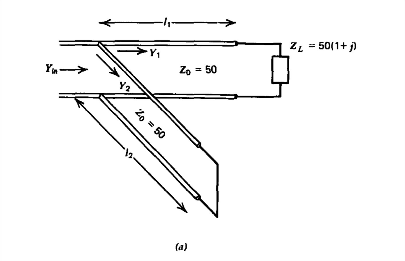
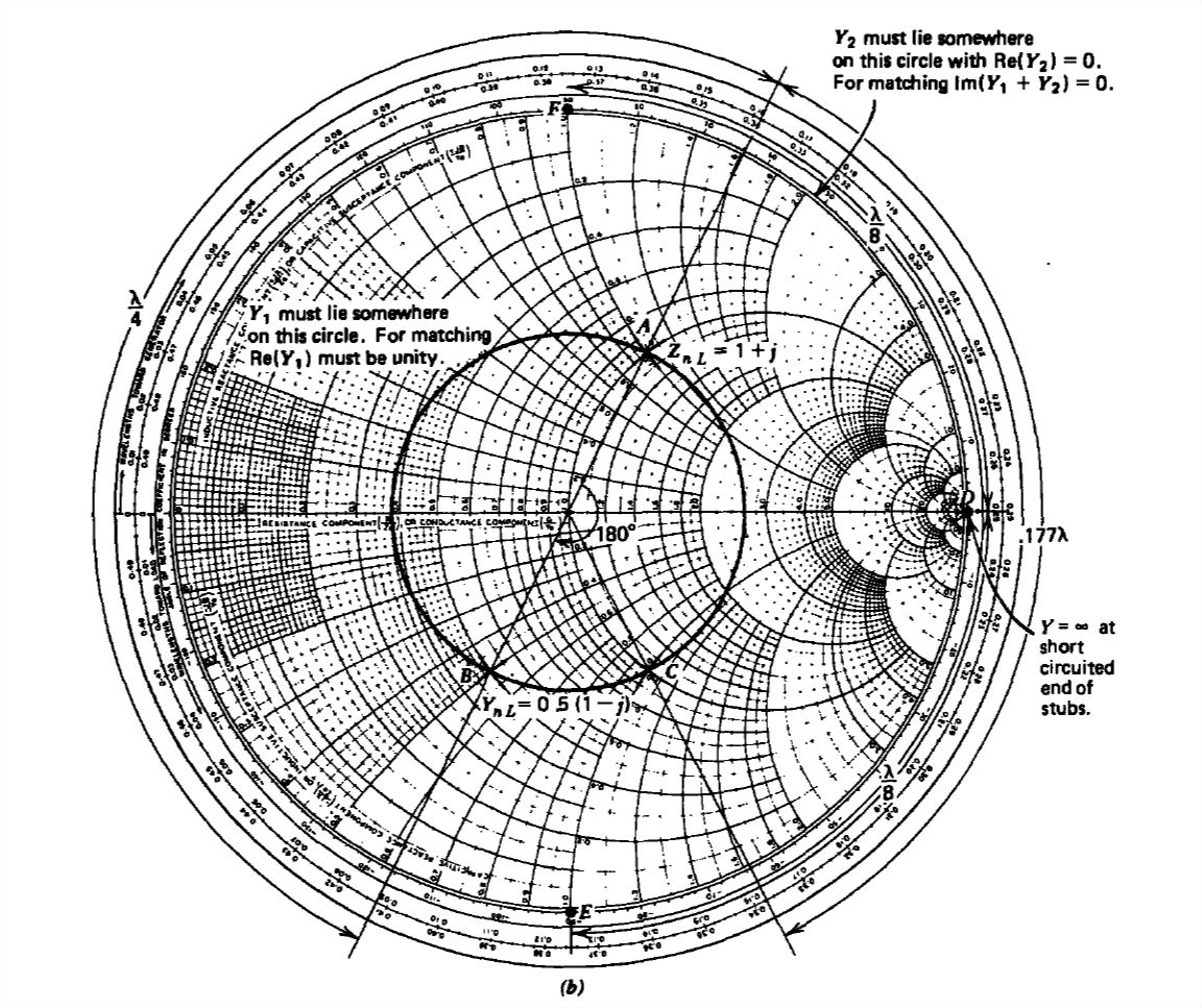
Figure 8-24 (a) A single stub tuner consisting of a variable length short circuited line $l_{2}$ can match any load to the line by putting the stub at the appropriate distance $l_{1}$, from the load. (b) Smith chart construction. (c) Voltage standing wave pattern.

Figure 8-24

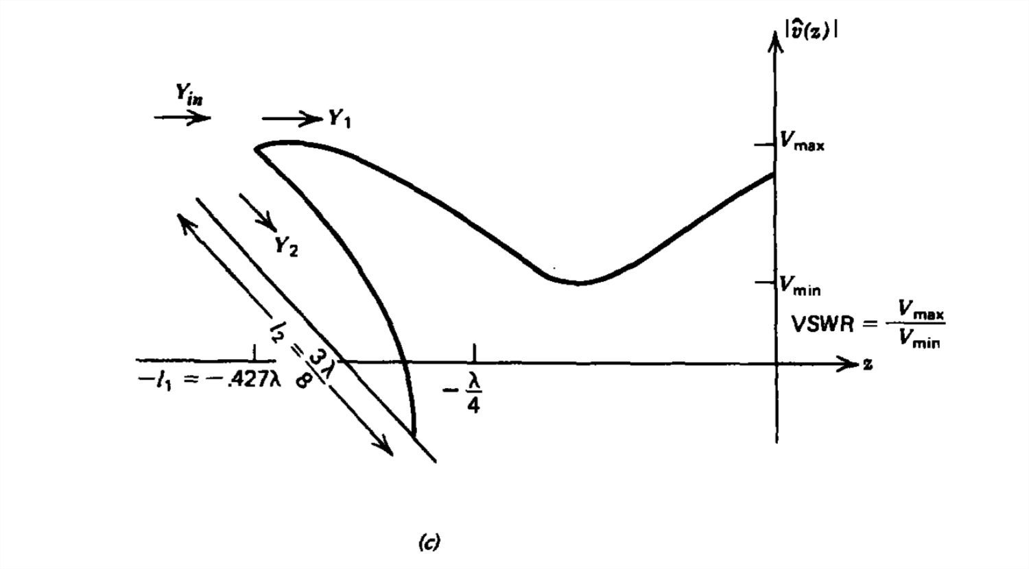
When the load is matched by the stub to the line, the $\textrm{VSWR}$ to the left of the stub is unity, while to the right of the stub over the length $l_{1}$ the reflection coefficient is

$$\Gamma _{L}=\frac{Z_{nL}-1}{Z_{nL}+1}=\frac{j}{2+j}$$

which has magnitude

$$\left |\Gamma _{L}  \right |=1/\sqrt{5}\approx 0.447$$

so that the voltage standing wave ratio is

$$\textrm{VSWR}=\frac{1+\left |\Gamma _{L} \right |}{1-\left |\Gamma _{L} \right |}\approx 2.62$$

The disadvantage to single-stub tuning is that it is not easy to vary the length $l_{1}$. Generally new elements can only be connected at the ends of the line and not inbetween.

Double-Stub Matching

This difficulty of not having a variable length line can be overcome by using two short circuited stubs a fixed length apart, as shown in Figure 8-25a. This fixed length is usually $\frac{3}{8}\lambda$. A match is made by adjusting the length of the stubs $l_{1}$ and

Figure 8-25 (a) A double stub tuner of fixed spacing cannot match all loads but is useful because additional elements can only be placed at transmission line terminations and not at any general position along a line as required for a single-stub tuner. (b) Smith chart construction. If the stubs are $\frac{3}{8}\lambda$ apart, normalized load admittances whose real part exceeds $2$ cannot be matched.

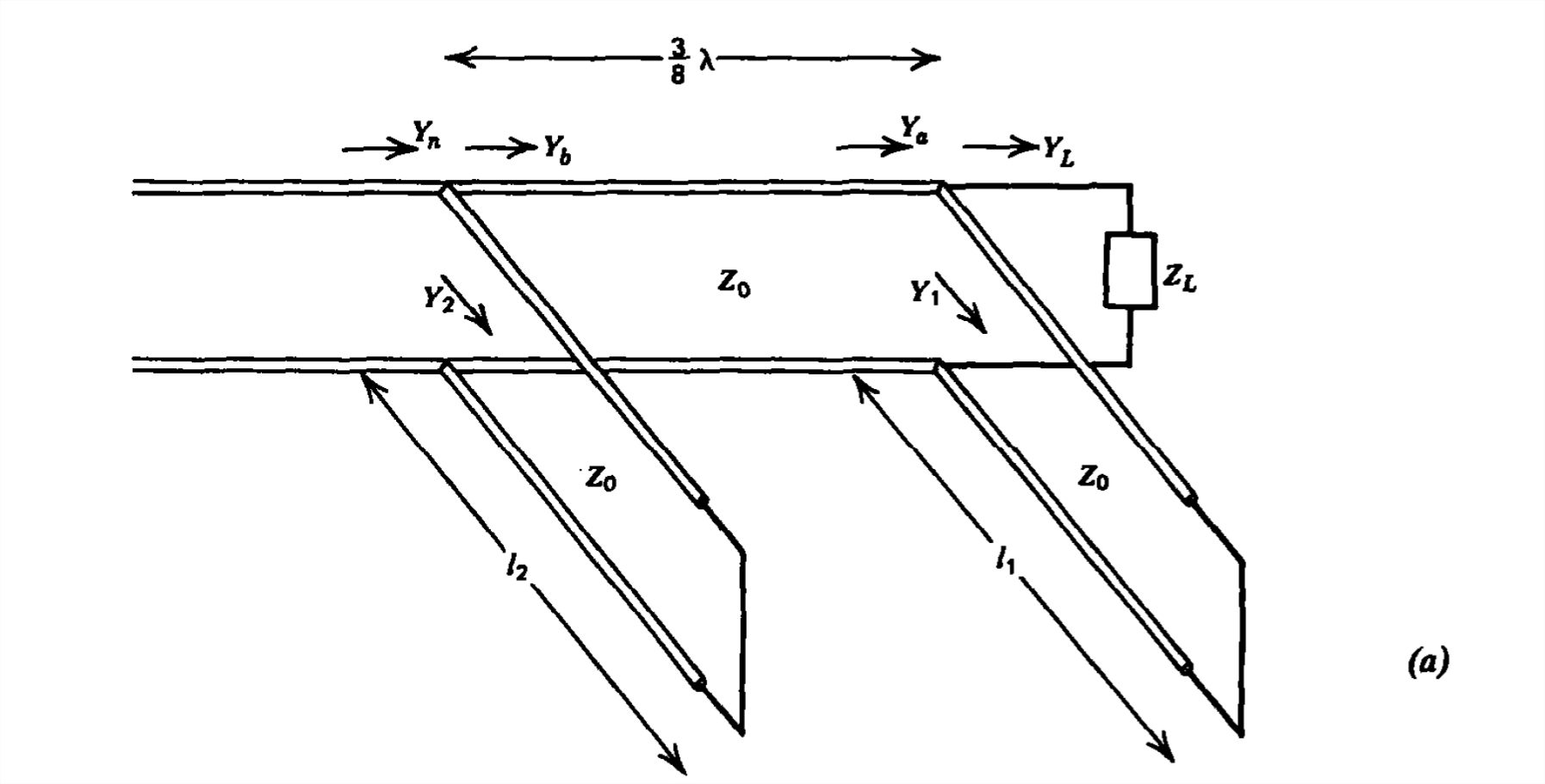
\$l_{2}$. One problem with the double-stub tuner is that not all loads can be matched for a given stub spacing.

The normalized admittances at each junction are related as

$$Y_{a}=Y_{1}+Y_{L}\\ Y_{n}=Y_{2}+Y_{b}$$

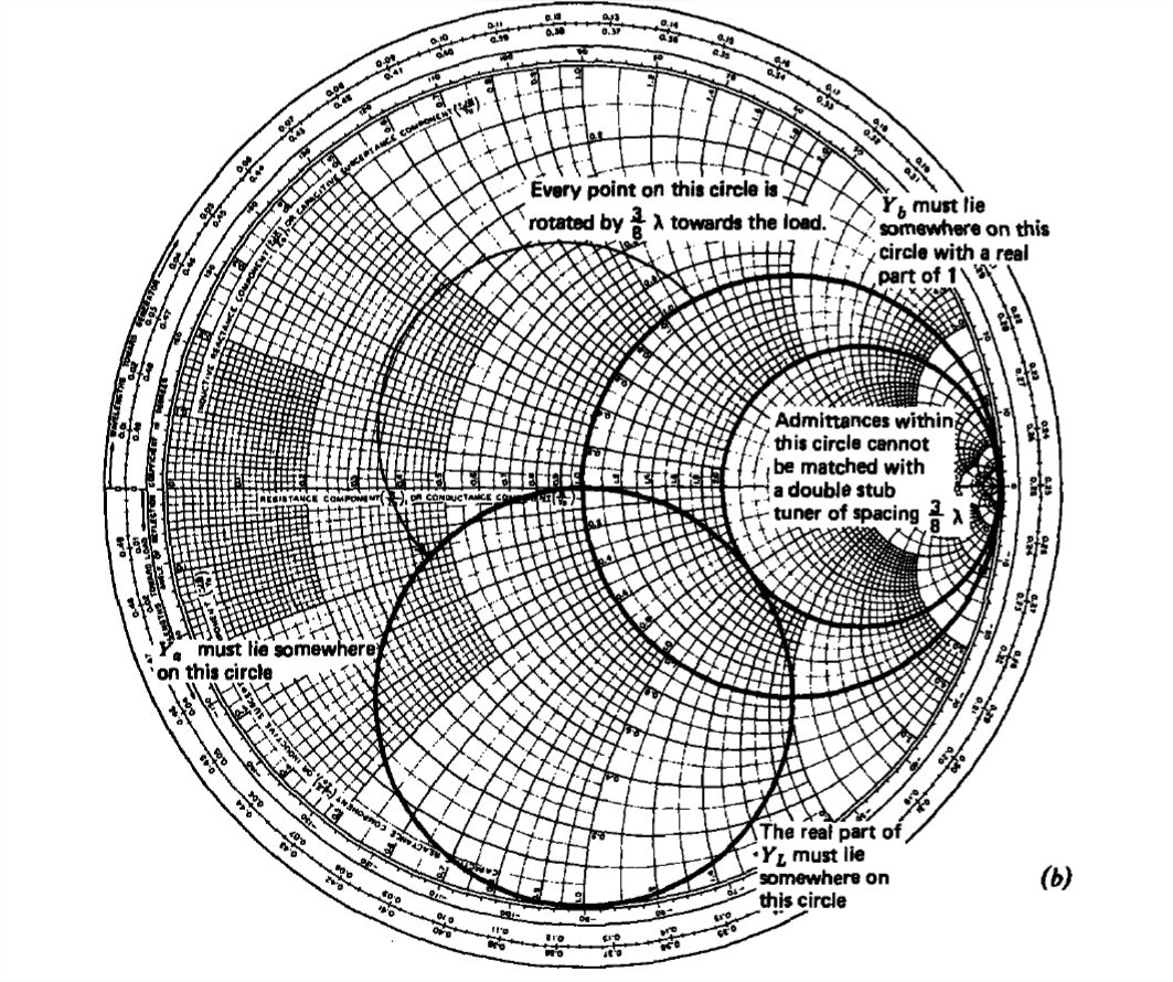
where $Y_{1}$ and $Y_{2}$ are the purely reactive admittances of the stubs reflected back to the junctions while $Y_{b}$ is the admittance of $Y_{a}$ reflected back towards the load by $\frac{3}{8}\lambda$. For a match we require that $Y_{n}$ be unity. Since $Y_{2}$ is purely imaginary, the real part of $Y_{b}$ must lie on the circle with a real part of unity. Then $Y_{a}$ must lie somewhere on this circle when each point on the circle is reflected back by $\frac{3}{8}\lambda$. This generates another circle that is $\frac{3}{2}\pi$ back in the counterclockwise direction as we are moving toward the load, as illustrated in Figure 8-25b. To find the conditions for a match, we work from left to right towards the load using the following reasoning:

1. Since $Y_{2}$ is purely imaginary, the real part of $Y_{b}$ must lie on the circle with a real part of unity, as in Figure 8-25b.
2. Every possible point on $Y_{b}$ must be reflected towards the load by $\frac{3}{8}\lambda$ to find the locus of possible match for $Y_{a}$. This generates another circle that is $\frac{3}{2}\pi$ back in the counterclockwise direction as we move towards the load, as in Figure 8-25b.

Again since $Y_{1}$ is purely imaginary, the real part of $Y_{a}$ must also equal the real part of the load admittance. This yields two possible solutions if the load admittance is outside the forbidden circle enclosing all load admittances with a real part greater than $2$. Only loads with normalized admittances whose real part is less than $2$ can be matched by the double-stub tuner of $\frac{3}{8}\lambda$ spacing. Of course, if a load is within the forbidden circle, it can be matched by a double-stub tuner if the stub spacing is different than $\frac{3}{8}\lambda$.

Example $\PageIndex{1}$ EXAMPLE 8-4 DOUBLE-STUB MATCHING

The load impedance $Z_{L}=50\left ( 1+j \right )$ on a $50$-$\textrm{Ohm}$ line is to be matched by a double-stub tuner of $\frac{3}{8}\lambda$ spacing. What stub lengths $l_{1}$ and $l_{2}$ are necessary?

SOLUTION

The normalized load impedance $Z_{nL}=1+j$ corresponds to a normalized load admittance:

$Y_{nL}=0.5\left ( 1-j \right )$

Figure 8-26 (a) The Smith chart construction for a double-stub tuner of $\frac{3}{8}\lambda$ spacing with $Z_{nL}=1+j$. (b) The voltage standing wave pattern.

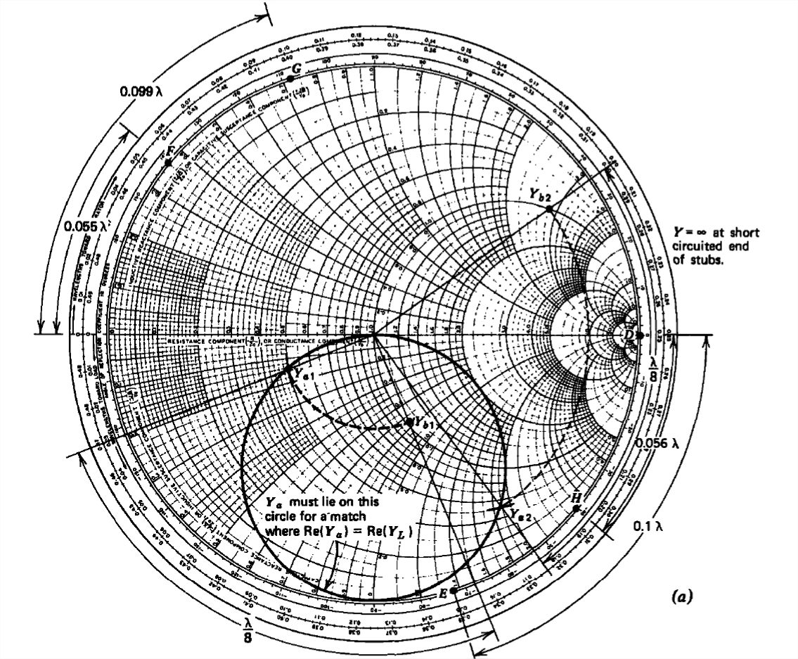
Then the two solutions for $Y_{a}$ lie on the intersection of the circle shown in Figure 8-26a with the $r = 0.5 \, \textrm{circle}$:

$Y_{a1}=0.5-0.14j\\ Y_{a2}=0.5-1.85j$

We then find $Y_{1}$ by solving for the imaginary part of the upper equation in (13):

$Y_{1}=j\textrm{Im}\left ( Y_{a}-Y_{L} \right )=\left\{\begin{matrix} 0.36j\Rightarrow l_{1}=0.305\lambda \,\left ( F \right )\\  -1.35j\Rightarrow l_{1}=0.1\lambda\,\left ( E \right ) \end{matrix}\right.$

By rotating the $Y_{a}$ solutions by $\frac{3}{8}\lambda$ back to the generator ($270^{\circ }$ clockwise, which is equivalent to $90^{\circ }$ counterclockwise), their intersection with the $r = 1$ circle gives the solutions for $Y_{b}$ as

$Y_{b1}=1.0-0.72j\\ Y_{b2}=1.0+2.7j$

This requires $Y_{2}$ to be

$Y_{2}=-j\textrm{Im}\left ( Y_{b}\right )=\left\{\begin{matrix} 0.72j\Rightarrow l_{2}=0.349\lambda \,\left ( G \right )\\  -2.7j\Rightarrow l_{2}=0.056\lambda\,\left ( H \right ) \end{matrix}\right.$

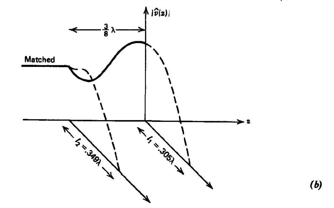
The voltage standing wave pattern along the line and stubs is shown in Figure 8.26b. Note the continuity of voltage at the junctions. The actual stub lengths can be those listed plus any integer multiple of $\lambda /2$.