8.6: The Rectangular Waveguide

We showed in Section 8-1-2 that the electric and magnetic fields for \(\textrm{TEM}\) waves have the same form of solutions in the plane transverse to the transmission line axis as for statics. The inner conductor within a closed transmission line structure such as a coaxial cable is necessary for \(\textrm{TEM}\) waves since it carries a surface current and a surface charge distribution, which are the source for the magnetic and electric fields. A hollow conducting structure, called a waveguide, cannot propagate \(\textrm{TEM}\) waves since the static fields inside a conducting structure enclosing no current or charge is zero.

However, new solutions with electric or magnetic fields along the waveguide axis as well as in the transverse plane are allowed. Such solutions can also propagate along transmission lines. Here the axial displacement current can act as a source of the transverse magnetic field giving rise to transverse magnetic (\(\textrm{TM}\)) modes as the magnetic field lies entirely within the transverse plane. Similarly, an axial time varying magnetic field generates transverse electric (\(\textrm{TE}\)) modes. The most general allowed solutions on a transmission line are \(\textrm{TEM}\), \(\textrm{TM}\), and \(\textrm{TE}\) modes. Removing the inner conductor on a closed transmission line leaves a waveguide that can only propagate \(\textrm{TM}\) and \(\textrm{TE}\) modes.

Governing Equations

To develop these general solutions we return to Maxwell's equations in a linear source-free material:

\[ \begin{align}\nabla \times \textbf{E}&=-\mu \frac{\partial \textbf{H}}{\partial t} \\
\nabla \times \textbf{H}&=\varepsilon \frac{\partial \textbf{E}}{\partial t} \nonumber \\
\varepsilon \nabla \cdot  \textbf{E}&=0 \nonumber \\
\mu  \nabla \cdot  \textbf{H}&=0 \nonumber \end{align} \]

Taking the curl of Faraday's law, we expand the double cross product and then substitute Ampere's law to obtain a simple vector equation in \(\textbf{E}\) alone:

\begin{align}\nabla \times \left ( \nabla \times \textbf{E} \right )&=\nabla\left ( \nabla \cdot \textbf{E} \right )-\nabla^{2}\textbf{E} \\&
=-\mu \frac{\partial }{\partial t}\left ( \nabla \times \textbf{H} \right ) \nonumber \\&
=-\varepsilon \mu \frac{\partial^2 \textbf{E}}{\partial t^2} \nonumber \end{align}

Since \(\nabla \cdot  \textbf{E}=0\) from Gauss's law when the charge density is zero, (2) reduces to the vector wave equation in \(\textbf{E}\):

\[ \nabla^{2}\textbf{E}=\frac{1}{c^{2}}\frac{\partial^2 \textbf{E}}{\partial t^2},\quad c^{2}=\frac{1}{\varepsilon \mu } \]

If we take the curl of Ampere's law and perform similar operations, we also obtain the vector wave equation in \(\textbf{H}\):

\[ \nabla^{2}\textbf{H}=\frac{1}{c^{2}}\frac{\partial^2 \textbf{H}}{\partial t^2} \]

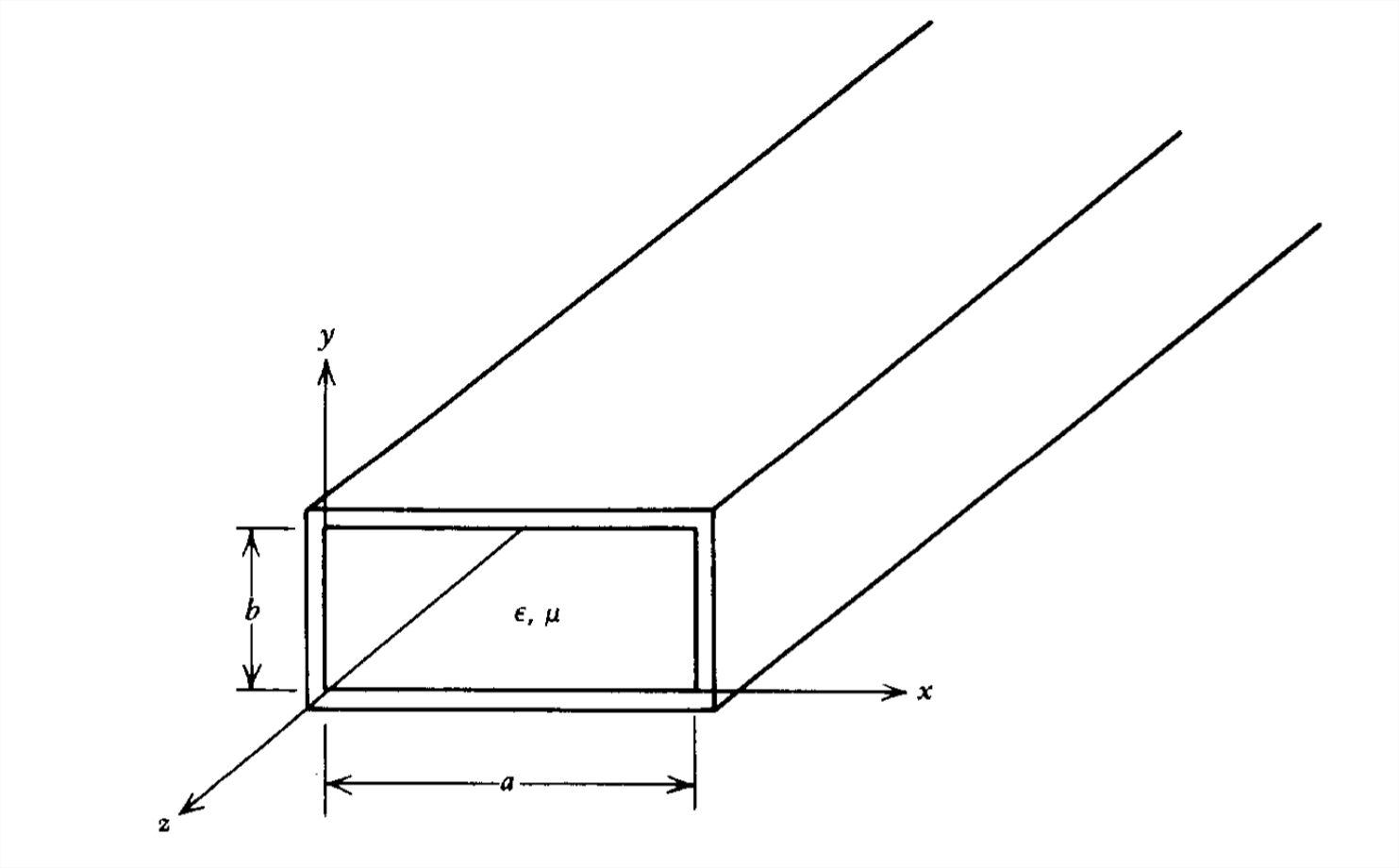
The solutions for \(\textbf{E}\) and \(\textbf{H}\) in (3) and (4) are not independent. If we solve for either \(\textbf{E}\) or \(\textbf{H}\), the other field is obtained from (1). The vector wave equations in (3) and (4) are valid for any shaped waveguide. In particular, we limit ourselves in this text to waveguides whose cross-sectional shape is rectangular, as shown in Figure 8-27.

Transverse Magnetic (TM) Modes

We first consider \(\textrm{TM}\) modes where the magnetic field has \(x\) and \(y\) components but no \(z\) component. It is simplest to solve (3) for the \(z\) component of electric field and then obtain the other electric and magnetic field components in terms of \(E_{z}\) directly from Maxwell's equations in (1).

We thus assume solutions of the form

\[ E_{z}=\textrm{Re}\left [ \hat{E}_{z}\left ( x,y \right )e^{j\left ( \omega t-k_{z}z \right )} \right ] \]

where an exponential \(z\) dependence is assumed because the cross-sectional area of the waveguide is assumed to be uniform in \(z\) so that none of the coefficients in (1) depends on \(z\). Then substituting into (3) yields the Helmholtz equation:

\[ \frac{\partial^2 E_{z}}{\partial x^2}+\frac{\partial^2 E_{z}}{\partial y^2}-\left ( k_{z}^{2}-\frac{\omega ^{2}}{c^{2}} \right )\hat{E}_{z}=0 \]

Figure 8-27 A lossless waveguide with rectangular cross section.

This equation can be solved by assuming the same product solution as used for solving Laplace's equation in Section 4-2-1, of the form

\[ \hat{E}_{z}\left ( x,y \right )=X\left ( x \right )Y\left ( y \right ) \]

where \(X\left ( x \right )\) is only a function of the \(x\) coordinate and \(Y\left ( y \right )\) is only a function of \(y\). Substituting this assumed form of solution into (6) and dividing through by \(X\left ( x \right )Y\left ( y \right )\) yields

\[ \frac{1}{X}\frac{d^{2}X}{dx^{2}}+\frac{1}{Y}\frac{d^{2}Y}{dy^{2}}=k_{z}^{2}-\frac{\omega ^{2}}{c^{2}} \]

When solving Laplace's equation in Section 4-2-1 the right-hand side was zero. Here the reasoning is the same. The first term on the left-hand side in (8) is only a function of \(x\) while the second term is only a function of \(y\). The only way a function of \(x\) and a function of \(y\) can add up to a constant for all \(x\) and \(y\) is if each function alone is a constant,

\[ \frac{1}{X}\frac{d^{2}X}{dx^{2}}=-k_{x}^{2}\\
\frac{1}{Y}\frac{d^{2}Y}{dy^{2}}=-k_{y}^{2} \]

where the separation constants must obey the relation

\[ k_{x}^{2}+k_{y}^{2}+k_{z}^{2}=k^{2}=\omega ^{2}/c^{2} \]

When we solved Laplace's equation in Section 4-2-6, there was no time dependence so that \(\omega =0\). Then we found that at least one of the wavenumbers was imaginary, yielding decaying solutions. For finite frequencies it is possible for all three wavenumbers to be real for pure propagation. The values of these wavenumbers will be determined by the dimensions of the waveguide through the boundary conditions.

The solutions to (9) are sinusoids so that the transverse dependence of the axial electric field \(\hat{E}_{z}\left ( x,y \right )\) is

\[ \hat{E}_{z}\left ( x,y \right )=\left ( A_{1}\sin k_{x}x+A_{2}\cos k_{x}x \right )\left ( B_{1}\sin k_{y}y+B_{2}\cos k_{y}y \right ) \]

Because the rectangular waveguide in Figure 8-27 is composed of perfectly conducting walls, the tangential component of electric field at the walls is zero:

\[ \hat{E}_{z}\left ( x,y=0 \right )=0,\quad \hat{E}_{z}\left ( x=0,y \right )=0\\
\hat{E}_{z}\left ( x,y=b \right )=0,\quad \hat{E}_{z}\left ( x=a,y \right )=0 \]

These boundary conditions then require that \(A_{2}\) and \(B_{2}\) are zero so that (11) simplifies to

\[ \hat{E}_{z}\left ( x,y \right )=E_{0}\sin k_{x}x\sin k_{y}y \]

where \(E_{0}\) is a field amplitude related to a source strength and the transverse wavenumbers must obey the equalities

\[ k_{x}=m\pi /a,\quad m=1,2,3,...\\
k_{y}=m\pi /b,\quad n=1,2,3,... \]

Note that if either \(m\) or \(n\) is zero in (13), the axial electric field is zero. The waveguide solutions are thus described as \(\textrm{TM}_{mn}\) modes where both \(m\) and \(n\) are integers greater than zero.

The other electric field components are found from the \(z\) component of Faraday's law, where \(\textbf{H}_{z}=0\) and the charge-free Gauss's law in (1):

\[ \frac{\partial E_{y}}{\partial x}=\frac{\partial E_{x}}{\partial y}\\
\frac{\partial E_{x}}{\partial x}+\frac{\partial E_{y}}{\partial y}+\frac{\partial E_{z}}{\partial z}=0 \]

By taking \(\partial /\partial x\) of the top equation and \(\partial /\partial y\) of the lower equation, we eliminate \(E_{x}\) to obtain

\[ \frac{\partial^2 E_{y}}{\partial x^2}+\frac{\partial^2 E_{y}}{\partial y^2}=-\frac{\partial^2 E_{z}}{\partial y\partial z} \]

where the right-hand side is known from (13). The general solution for \(E_{y}\) must be of the same form as (11), again requiring the tangential component of electric field to be zero at the waveguide walls,

\[ \hat{E}_{y}\left ( x=0,y \right )=0,\quad \hat{E}_{y}\left ( x=a,y \right )=0 \]

so that the solution to (16) is

\[ \hat{E}_{y}=-\frac{jk_{y}k_{z}E_{0}}{k_{x}^{2}+k_{y}^{2}}\sin k_{x}x\cos k_{y}y \]

We then solve for \(E_{x}\) using the upper equation in (15):

\[ \hat{E}_{x}=-\frac{jk_{x}k_{z}E_{0}}{k_{x}^{2}+k_{y}^{2}}\cos k_{x}x\sin k_{y}y \]

where we see that the boundary conditions

\[ \hat{E}_{x}\left ( x,y=0 \right )=0,\quad \hat{E}_{x}\left ( x,y=b \right )=0  \]

are satisfied.

The magnetic field is most easily found from Faraday's law

\[ \hat{\textbf{H}}\left ( x,y \right )=-\frac{1}{j\omega \mu }\nabla \times \hat{\textbf{E}}\left ( x,y \right ) \]

to yield

\[ \begin{align}\hat{H}_{x}&=-\frac{1}{j\omega \mu }\left ( \frac{\partial \hat{E}_{z}}{\partial y}-\frac{\partial \hat{E}_{y}}{\partial z} \right ) \\ &
=-\frac{k_{y}k^{2}}{j\omega \mu \left ( k_{x}^{2}+k_{y}^{2} \right )}E_{0}\sin k_{x}x\cos k_{y}y \nonumber \\ &
=\frac{j\omega \varepsilon k_{y}}{k_{x}^{2}+k_{y}^{2}}E_{0}\sin k_{x}x\cos k_{y}y \nonumber \\ 
\hat{H}_{y}&=-\frac{1}{j\omega \mu }\left ( \frac{\partial \hat{E}_{x}}{\partial z}-\frac{\partial \hat{E}_{z}}{\partial x} \right ) \nonumber \\ &
=\frac{k_{y}k^{2}E_{0}}{j\omega \mu \left ( k_{x}^{2}+k_{y}^{2} \right )}\cos k_{x}x\sin k_{y}y \nonumber \\ &
=-\frac{j\omega \varepsilon k_{x}}{k_{x}^{2}+k_{y}^{2}}E_{0}\cos k_{x}x\sin k_{y}y \nonumber \\ 
\hat{H}_{z}&=0 \nonumber \end{align}  \]

Note the boundary conditions of the normal component of \(\textbf{H}\) being zero at the waveguide walls are automatically satisfied:

\[ \hat{H}_{y}\left ( x,y=0 \right )=0,\quad \hat{H}_{y}\left ( x,y=b \right )=0\\
\hat{H}_{x}\left ( x=0,y \right )=0,\quad \hat{H}_{y}\left ( x=a,y \right )=0  \]

The surface charge distribution on the waveguide walls is found from the discontinuity of normal \(\textbf{D}\) fields:

\[\]\[ \hat{\sigma }_{f}\left ( x=0,y \right )=\varepsilon \hat{E}_{x}\left ( x=0,y \right )=-\frac{jk_{z}k_{x}\varepsilon }{k_{x}^{2}+k_{y}^{2}}E_{0}\sin k_{y}y \nonumber \\
\hat{\sigma }_{f}\left ( x=a,y \right )=-\varepsilon \hat{E}_{x}\left ( x=a,y \right )=\frac{jk_{z}k_{x}\varepsilon }{k_{x}^{2}+k_{y}^{2}}E_{0}\cos m\pi \sin k_{y}y \nonumber \\
\hat{\sigma }_{f}\left ( x,y=0 \right )=\varepsilon \hat{E}_{x}\left ( x,y=0 \right )=-\frac{jk_{z}k_{y}\varepsilon }{k_{x}^{2}+k_{y}^{2}}E_{0}\sin k_{x}x \nonumber \\
\hat{\sigma }_{f}\left ( x,y=b \right )=-\varepsilon \hat{E}_{x}\left ( x,y=0 \right )=-\frac{jk_{z}k_{y}\varepsilon }{k_{x}^{2}+k_{y}^{2}}E_{0}\cos n\pi \sin k_{x}x \nonumber \]

Similarly, the surface currents are found by the discontinuity in the tangential components of \(\textbf{H}\) to be purely \(z\) directed:

\[\]\[ \hat{K}_{z}\left ( x,y=0 \right )=-\hat{H}_{x}\left ( x,y=0 \right )=\frac{k_{y}k^{2}E_{0}\sin k_{x}x}{j\omega \mu \left (k_{x}^{2}+k_{y}^{2}  \right )} \nonumber \\ 
\hat{K}_{z}\left ( x,y=b \right )=\hat{H}_{x}\left ( x,y=b \right )=-\frac{k_{y}k^{2}E_{0}}{j\omega \mu \left (k_{x}^{2}+k_{y}^{2}  \right )}\sin k_{x}x\cos n\pi \nonumber \\
\hat{K}_{z}\left ( x=0,y \right )=\hat{H}_{x}\left ( x,y=0 \right )=\frac{k_{x}k^{2}E_{0}}{j\omega \mu \left (k_{x}^{2}+k_{y}^{2}  \right )}\sin k_{y}y \nonumber \\  
\hat{K}_{z}\left ( x=a,y \right )=-\hat{H}_{x}\left ( x=a,y \right )=-\frac{k_{x}k^{2}E_{0}\cos m\pi \sin k_{y}y}{j\omega \mu \left (k_{x}^{2}+k_{y}^{2}  \right )}  \nonumber \]

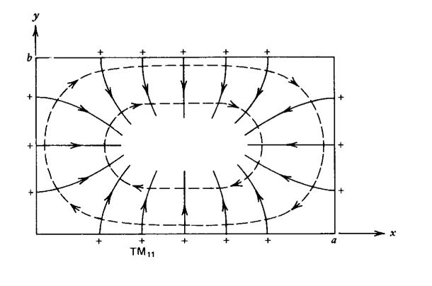
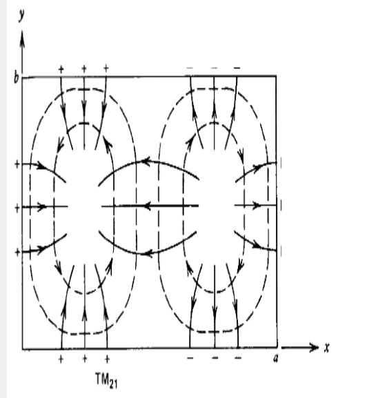
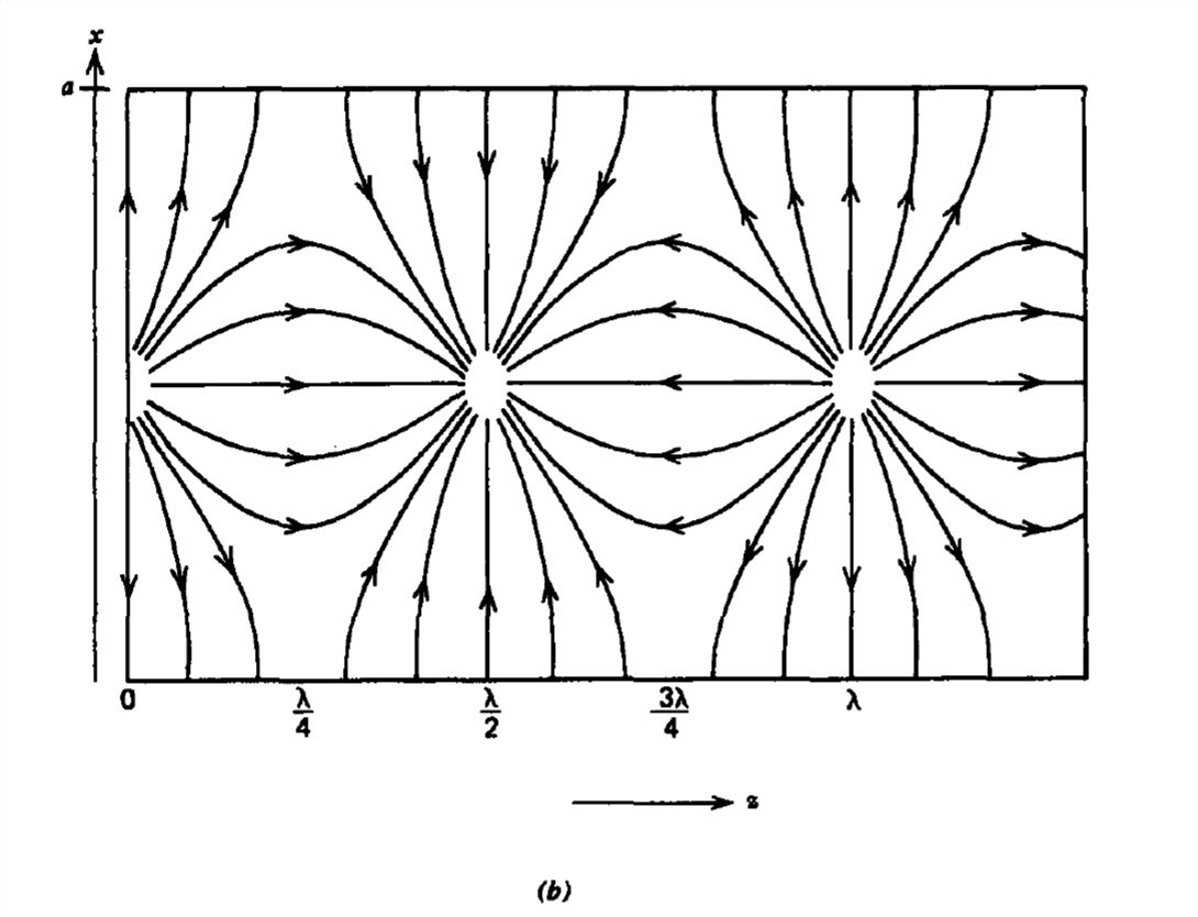
We see that if \(m\) or \(n\) are even, the surface charges and surface currents on opposite walls are of opposite sign, while if \(m\) or \(n\) are odd, they are of the same sign. This helps us in plotting the field lines for the various \(\textrm{TM}_{mn}\). modes shown in Figure 8-28. The electric field is always normal and the magnetic field tangential to the waveguide walls. Where the surface charge is positive, the electric field points out of the wall, while it points in where the surface charge is negative. For higher order modes the field patterns shown in Figure 8-28 repeat within the waveguide.

Slots are often cut in waveguide walls to allow the insertion of a small sliding probe that measures the electric field. These slots must be placed at positions of zero surface current so that the field distributions of a particular mode are only negligibly disturbed. If a slot is cut along the \(z\) direction on the \(y = b\) surface at \(x = a/2\), the surface current given in (25) is zero for \(\textrm{TM}\) modes if \(\sin \left ( k_{x}a/2 \right )=0\), which is true for the \(m=\textrm{even}\) modes.

Transverse Electric (TE) Modes

When the electric field lies entirely in the \(xy\) plane, it is most convenient to first solve (4) for \(H_{z}\). Then as for \(\textrm{TM}\) modes we assume a solution of the form

\[ H_{z}=\textrm{Re}\left [ \hat{H}_{z}\left ( x,y \right )e^{j\left (\omega t-k_{z}z  \right )} \right ] \]

which when substituted into (4) yields

\[ \frac{\partial^2 \hat{H}_{z}}{\partial x^2}+\frac{\partial^2 \hat{H}_{z}}{\partial y^2}-\left ( k_{z}^{2}-\frac{\omega ^{2}}{c^{2}} \right )\hat{H}_{z}=0 \]

 

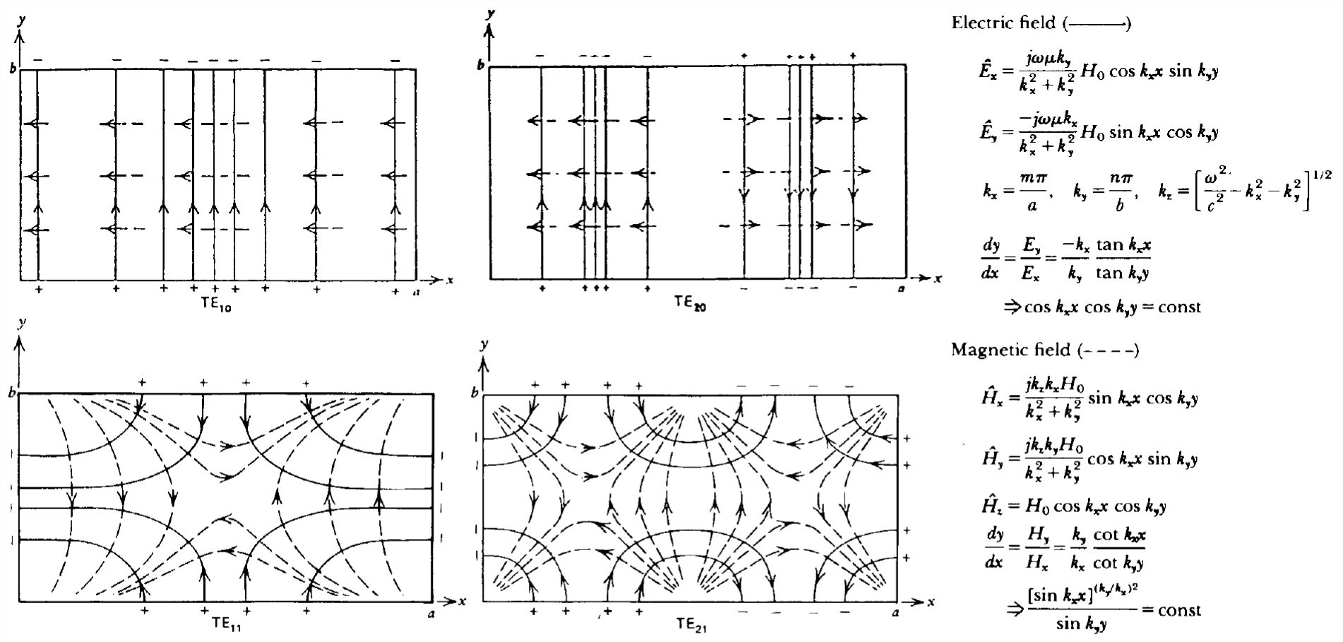
Electric field ( \(\longrightarrow\) ) \begin{array}{l} \hat{E}_x=\frac{-j k_x k_z E_0}{k_x^2+k_y^2} \cos k_x x \sin k_y y \nonumber \\ \hat{E}_y=\frac{-j k_y k_z E_0}{k_x^2+k_y^2} \sin k_x x \cos k_y y \nonumber\\ \hat{E}_x=E_0 \sin k_x x \sin k_y y \nonumber\\ \frac{d y}{d x}=\frac{E_y}{E_x}=\frac{k_y}{k_x} \frac{\tan k_x x}{\tan k_y y} \nonumber\\ \Rightarrow \frac{\left[\cos k_x x\right]^{\left(k_y / k_x\right)^2}}{\cos k_y y}=\text { const } \nonumber \end{array}

Magnetic field (- - - ) \[ \begin{array}{c} \hat{H}_x=\frac{j \omega \varepsilon k_y}{k_x^2+k_y^2} E_0 \sin k_x x \cos k_y y \nonumber  \\ \hat{H}_y=\frac{-j \omega \varepsilon k_x}{k_x^2+k_y^2} E_0 \cos k_x x \sin k_y y \nonumber \\ \frac{d y}{d x}=\frac{H_y}{H_x}=\frac{-k_x \cot k_x x}{k_y \cot k_y y} \nonumber \\ \Rightarrow \sin k_x x \sin k_y y=\operatorname{const} \nonumber \\ k_x=\frac{m \pi}{a}, \quad k_y=\frac{n \pi}{b}, \quad k_x=\left[\frac{\omega^2}{c^2}- k_{x}^2 - k_{y}^2 \right]^{1/2}. \nonumber \end{array} \]

Figure 8-28 The transverse electric and magnetic field lines for the \(\textrm{TM}_{11}\) and \(\textrm{TM}_{21}\) modes. The electric field is purely \(z\) directed where the field lines converge.

Again this equation is solved by assuming a product solution and separating to yield a solution of the same form as (11):

\[ \hat{H}_{z}\left ( x,y \right )=\left ( A_{1}\sin k_{x}x+A_{2}\cos k_{x}x \right )\left ( B_{1}\sin k_{y}y+B_{2}\cos k_{y}y \right ) \]

The boundary conditions of zero normal components of \(\)H at the waveguide walls require that

\[\]\[ \hat{H}_{x}\left ( x=0,y \right )=0,\quad \hat{H}_{x}\left ( x=a,y \right )=0 \nonumber \\
\hat{H}_{y}\left ( x,y=0 \right )=0,\quad \hat{H}_{y}\left ( x,y=b \right )=0 \nonumber \]

Using identical operations as in (15)-(20) for the \(\textrm{TM}\) modes the magnetic field solutions are

\[ \begin{align}\hat{H}_{x}&=\frac{jk_{z}k_{x}H_{0}}{k_{x}^{2}+k_{y}^{2}}\sin k_{x}x\cos k_{y}y,\quad k_{x}=\frac{m\pi }{a},\,k_{y}=\frac{n\pi }{b} \\
\hat{H}_{y}&=\frac{jk_{z}k_{y}H_{0}}{k_{x}^{2}+k_{y}^{2}}\sin k_{x}x\cos k_{y}y \nonumber \\
\hat{H}_{z}&=H_{0}\cos k_{x}x\cos k_{y}y \nonumber \end{align} \]

The electric field is then most easily obtained from Ampere's law in (1),

\[ \hat{\textbf{E}}=\frac{1}{j\omega \varepsilon }\nabla \times \hat{\textbf{H}} \]

to yield

\[ \begin{align}\hat{E}_{x}&=\frac{1}{j\omega\varepsilon }\left ( \frac{\partial }{\partial y}\hat{H}_{z}-\frac{\partial }{\partial z}\hat{H}_{y} \right ) \\ &  
=-\frac{k_{y}k^{2}H_{0}}{j\omega\varepsilon \left ( k_{x}^{2}+k_{y}^{2} \right )}\cos k_{x}x\sin k_{y}y \nonumber \\ &
=\frac{j\omega\mu  k_{y}}{k_{x}^{2}+k_{y}^{2}}H_{0}\cos k_{x}x \sin k_{y}y \nonumber \\  
\hat{E}_{y}&=\frac{1}{j\omega \varepsilon }\left ( \frac{\partial \hat{H}_{x}}{\partial z}-\frac{\partial \hat{H}_{z}}{\partial x} \right ) \nonumber \\ &  
=\frac{k_{x}k^{2}H_{0}}{j\omega \varepsilon  \left ( k_{x}^{2}+k_{y}^{2} \right )}\sin k_{x}x\cos k_{y}y \nonumber \\ &
=-\frac{j\omega \mu k_{x}}{k_{x}^{2}+k_{y}^{2}}H_{0}\sin k_{x}x\cos k_{y}y \nonumber \\ 
\hat{E}_{z}&=0 \nonumber \end{align} \]

We see in (32) that as required the tangential components of the electric field at the waveguide walls are zero. The surface charge densities on each of the walls are:

\[\]\[ \hat{\sigma }_{f}\left ( x=0,y \right )=\varepsilon \hat{E}_{x}\left ( x=0,y \right )=\frac{-k_{y}k^{2}H_{0}}{j\omega \left (k_{x}^{2}+k_{y}^{2}  \right )}\sin k_{y}y \nonumber \\ 
\hat{\sigma }_{f}\left ( x=a,y \right )=-\varepsilon \hat{E}_{x}\left ( x=a,y \right )=\frac{k_{y}k^{2}H_{0}}{j\omega \left (k_{x}^{2}+k_{y}^{2}  \right )}\cos m\pi \sin k_{y}y \nonumber \\
\hat{\sigma }_{f}\left ( x,y=0 \right )=\varepsilon \hat{E}_{y}\left ( x,y=0 \right )=-\frac{k_{x}k^{2}H_{0}}{j\omega \left (k_{x}^{2}+k_{y}^{2}  \right )}\sin k_{x}x \nonumber \\ 
\hat{\sigma }_{f}\left ( x,y=b \right )=-\varepsilon \hat{E}_{y}\left ( x,y=b \right )=-\frac{k_{x}k^{2}H_{0}}{j\omega \left (k_{x}^{2}+k_{y}^{2}  \right )}\cos n\pi \sin k_{x}x  \nonumber \]

For \(\textrm{TE}\) modes, the surface currents determined from the discontinuity of tangential \(\textbf{H}\) now flow in closed paths on the waveguide walls:

\[ \begin{align} \hat{\textbf{K}}\left ( x=0,y \right )&=\textbf{i}_{x}\times \hat{\textbf{H}}\left ( x=0,y \right ) \\ &
=\textbf{i}_{z}\hat{H}_{y}\left ( x=0,y \right )-\textbf{i}_{y}\hat{H}_{z}\left ( x=0,y \right ) \nonumber \\
\hat{\textbf{K}}\left ( x=a,y \right )&=-\textbf{i}_{x}\times \hat{\textbf{H}}\left ( x=a,y \right ) \nonumber \\&
=-\textbf{i}_{z}\hat{H}_{y}\left ( x=a,y \right )+\textbf{i}_{y}\hat{H}_{z}\left ( x=a,y \right ) \nonumber \\
\hat{\textbf{K}}\left ( x,y=0 \right )&=\textbf{i}_{y}\times \hat{\textbf{H}}\left ( x,y=0 \right ) \nonumber \\&
=-\textbf{i}_{z}\hat{H}_{x}\left ( x,y=0 \right )+\textbf{i}_{x}\hat{H}_{z}\left ( x,y=0 \right ) \nonumber \\
\hat{\textbf{K}}\left ( x,y=b \right )&=-\textbf{i}_{y}\times \hat{\textbf{H}}\left ( x,y=b \right ) \nonumber \\&
=\textbf{i}_{z}\hat{H}_{x}\left ( x,y=b \right )-\textbf{i}_{x}\hat{H}_{z}\left ( x,y=b \right ) \nonumber \end{align} \]

Note that for \(\textrm{TE}\) modes either \(n\) or \(m\) (but not both) can be zero and still yield a nontrivial set of solutions. As shown in Figure 8-29, when \(n\) is zero there is no variation in the fields in the \(y\) direction and the electric field is purely \(y\) directed while the magnetic field has no \(y\) component. The \(\textrm{TE}_{11}\) and \(\textrm{TE}_{21}\) field patterns are representative of the higher order modes.

Cut-Off

The transverse wavenumbers are

\[ k_{x}=\frac{m\pi }{a},\quad k_{y}=\frac{n\pi }{b} \]

so that the axial variation of the fields is obtained from (10) as

\[ k_{z}=\left [ \frac{\omega_{2}}{c^{2}}-k_{x}^{2}-k_{y}^{2} \right ]^{1/2}=\left [ \frac{\omega^{2}}{c^{2}}-\left ( \frac{m\pi }{a} \right )^{2}-\left ( \frac{n\pi }{b} \right )^{2} \right ]^{1/2} \]

Figure 8-29 (a) The transverse electric and magnetic field lines for various \(\textrm{TE}\) modes. The magnetic field is purely \(z\) directed where the field lines converge. The \(\textrm{TE}_{10}\) mode is called the dominant mode since it has the lowest cut-off frequency. (b) Surface current lines for the \(\textrm{TE}_{10}\) mode.

Figure 8-29

Thus, although \(k_{x}\) and \(k_{y}\) are real, \(k_{z}\) can be either pure real or pure imaginary. A real value of \(k_{z}\) represents power flow down the waveguide in the z direction. An imaginary value of \(k_{z}\) means exponential decay with no time-average power flow. The transition from propagating waves (\(k_{z}\) real) to evanescence (\(k_{z}\) imaginary) occurs for \(k_{z}=0\). The frequency when is zero is called the cut-off frequency \(\omega _{c}\):

\[ \omega _{c}=c\left [ \left ( \frac{m\pi }{a} \right )^{2}+\left ( \frac{n\pi }{b} \right )^{2} \right ]^{1/2} \]

This frequency varies for each mode with the mode parameters \(m\) and \(n\). If we assume that \(a\) is greater than \(b\), the lowest cut-off frequency occurs for the \(\textrm{TE}_{10}\) mode, which is called the dominant or fundamental mode. No modes can propagate below this lowest critical frequency \(\omega _{c0}\):

\[ \omega _{c0}=\frac{\pi c}{a}\Rightarrow f_{c0}=\frac{\omega _{c0}}{2\pi }=\frac{c}{2a}\textrm{Hz} \]

If an air-filled waveguide has \(a=1\,\textrm{cm}\), then \(f_{c0}=1.5\times 10^{10}\,\textrm{Hz}\), while if \(a=10\,\textrm{cm}\), then \(f_{c0}=15\,\textrm{MHz}\). This explains why we usually cannot hear the radio when driving through a tunnel. As the frequency is raised above \(\omega _{c0}\), further modes can propagate.

The phase and group velocity of the waves are

\[ v_{p}=\frac{\omega }{k_{z}}=\frac{\omega }{\left [ \frac{\omega^{2}}{c^{2}}-\left ( \frac{m\pi }{a} \right )^{2}-\left ( \frac{n\pi }{b} \right )^{2} \right ]^{1/2}}\\
v_{g}=\frac{d\omega }{dk_{z}}=\frac{k_{z}c^{2}}{\omega }=\frac{c^{2}}{v_{p}}\Rightarrow v_{g}v_{p}=c^{2}  \]

At cut-off, \(v_{g}=0\) and \(v_{p}=\infty \) with their product always a constant.

Waveguide Power Flow

The time-averaged power flow per unit area through the waveguide is found from the Poynting vector:

\[ <\textbf{S}>=\frac{1}{2}\textrm{Re}\left ( \hat{\textbf{E}}\times \hat{\textbf{H}}^{\ast }\right ) \]

(a) Power Flow for the TM Modes

Substituting the field solutions found in Section 8-6-2 into (40) yields

\[ \begin{align}<\textbf{S}>&=\frac{1}{2}\textrm{Re}\left [ \left ( \hat{E}_{x}\textbf{i}_{x}+\hat{E}_{y}\textbf{i}_{y}+\hat{E}_{z}\textbf{i}_{z} \right )e^{-jk_{z}z}\times  \left ( \hat{H}_{x}^{\ast }\textbf{i}_{x}+\hat{H}_{y}^{\ast }\textbf{i}_{y} \right )e^{+jk_{z}^{\ast }z}\right ] \\ &
=\frac{1}{2}\textrm{Re}\left [ \left ( \hat{E}_{x}\hat{H}_{y}^{\ast } -\hat{E}_{y}\hat{H}_{x}^{\ast }\right ) \textbf{i}_{z}+\hat{E}_{z}\left ( \hat{H}_{x}^{\ast }\textbf{i}_{y}-\hat{H}_{y}^{\ast }\textbf{i}_{x} \right )\right ]e^{-j\left (k_{z}-k_{z}^{\ast } \right )z} \nonumber \end{align} \]

where we remember that \(k_{z}\) may be imaginary for a particular mode if the frequency is below cut-off. For propagating modes where \(k_{z}\) is real so that \(k_{z}=k_{z}^{\ast }\), there is no \(z\) dependence in (41). For evanescent modes where \(k_{z}\) is pure imaginary, the z dependence of the Poynting vector is a real decaying exponential of the form \(e^{-2\left | k_{z} \right |z}\). For either case we see from (13) and (22) that the product of \(\hat{E}_{z}\) with ff. and \(\hat{H}_{x}\) is pure imaginary so that the real parts of the \(x\)- and \(y\)-directed time average power flow are zero in (41). Only the \(z\)-directed power flow can have a time average:

\[ <\textbf{S}>=\frac{\omega \varepsilon \left | E_{0} \right |^{2}}{2\left ( k_{x}^{2}+k_{y}^{2} \right )}\textrm{Re}\left [ k_{z}e^{-j\left ( k_{z}-k_{z}^{\ast }\right )z}\left ( k_{x}^{2}\cos ^{2}k_{x}x\sin ^{2} k_{y}y+ k_{y}^{2}\sin^{2}k_{x}x\cos^{2} k_{y}y\right ) \right ]\textbf{i}_{z} \]

If \(k_{z}\) is imaginary, we have that \(<\textbf{S}>=0\) while a real \(k_{z}\) results in a nonzero time-average power flow. The total \(z\)-directed power flow is found by integrating (42) over the cross-sectional area of the waveguide:

\[ \begin{align} <P>&=\int_{x=0}^{a}\int_{y=0}^{b} <S_{z}>dxdy \\ &
=\frac{\omega \varepsilon k_{z}abE_{0}^{2}}{8\left ( k_{x}^{2}+k_{y}^{2} \right )} \nonumber \end{align} \]

where it is assumed that \(k_{z}\) is real, and we used the following identities:

\[\]\[ \int_{0}^{a}\sin ^{2}\frac{m\pi x}{a}dx=\frac{a}{m\pi }\left ( \frac{1}{2}\frac{m\pi x}{a}-\frac{1}{4}\sin \frac{2m\pi x}{a} \right )\bigg|_{0}^{a}=\left\{\begin{matrix}
a/2,\quad m\neq 0\\ 
0,\quad m=0
\end{matrix}\right. \nonumber \\
\int_{0}^{a}\cos ^{2}\frac{m\pi x}{a}dx=\frac{a}{m\pi }\left ( \frac{1}{2}\frac{m\pi x}{a}+\frac{1}{4}\sin \frac{2m\pi x}{a} \right )\bigg|_{0}^{a}=\left\{\begin{matrix}
a/2,\quad m\neq 0 \nonumber \\ 
0,\quad m=0
\end{matrix}\right. \nonumber \]

For the \(\textrm{TM}\) modes, both m and n must be nonzero.

(b) Power Flow for the TE Modes

The same reasoning is used for the electromagnetic fields found in Section 8-6-3 substituted into (40):

\[ \begin{align}<\textbf{S}>&=\frac{1}{2}\textrm{Re}\left [ \left ( \hat{E}_{x}\textbf{i}_{x}+\hat{E}_{y}\textbf{i}_{y} \right )e^{-jk_{z}z}\times \left ( \hat{H}_{x}^{\ast }\textbf{i}_{x}+\hat{H}_{y}^{\ast }\textbf{i}_{y}+\hat{H}_{z}^{\ast }\textbf{i}_{z} \right )e^{+jk_{z}^{\ast }z} \right ] \\ &
=\frac{1}{2}\textrm{Re}\left [ \left ( \hat{E}_{x}\hat{H}_{y}^{\ast }-\hat{E}_{y}\hat{H}_{x}^{\ast } \right )\textbf{i}_{z}-\hat{H}_{z}^{\ast }\left (\hat{E}_{x}\textbf{i}_{y}-\hat{E}_{y}\textbf{i}_{x} \right ) \right ]e^{-j\left (k_{z}-k_{z}^{\ast } \right )z} \nonumber \end{align} \]

Similarly, again we have that the product of \(\hat{H}_{z}^{\ast }\) with \(\hat{E}_{x}\) and \(\hat{E}_{y}\) is pure imaginary so that there are no \(x\)-and \(y\)-directed time average power flows. The \(z\)-directed power flow reduces to

\[ <S_{z}>=\frac{1}{2}\frac{\omega \mu H_{0}^{2}}{\left ( k_{x}^{2}+k_{y}^{2} \right )}\left ( k_{y}^{2}\cos ^{2} k_{x}x\sin ^{2}k_{y}y+k_{x}^{2}\sin ^{2}k_{x}x\cos ^{2}k_{y}y\right )\textrm{Re}\left ( k_{z}e^{-j\left ( k_{z}-k_{z}^{\ast } \right )z} \right ) \]

Again we have nonzero \(z\)-directed time average power flow only if \(k_{z}\) is real. Then the total z-directed power is

\[ <P>=\int_{x=0}^{a}\int_{y=0}^{b}<S_{z}>dx\,dy=\left\{\begin{matrix}
\frac{\omega \mu k_{z}abH_{0}^{2}}{8\left ( k_{x}^{2}+k_{y}^{2} \right )},\quad m,n\neq 0\\ 
\frac{\omega \mu k_{z}abH_{0}^{2}}{4\left ( k_{x}^{2}+k_{y}^{2} \right )},\quad m\,\textrm{or}\,n\neq 0
\end{matrix}\right.  \]

where we again used the identities of (44). Note the factor of \(2\) differences in (47) for either the \(\textrm{TE}_{10}\) or \(\textrm{TE}_{01}\), modes. Both \(m\) and \(n\) cannot be zero as the \(\textrm{TE}_{00}\) mode reduces to the trivial spatially constant uncoupled \(z\)-directed magnetic field.

Wall Losses

If the waveguide walls have a high but noninfinite Ohmic conductivity \(\sigma _{w}\), we can calculate the spatial attenuation rate using the approximate perturbation approach described in Section 8-3-4b. The fields decay as \(e^{-\alpha z}\), where

\[ \alpha =\frac{1}{2}\frac{<P_{dL}>}{<P>} \]

where \(<P_{dL}>\) is the time-average dissipated power per unit length and \(<P>\) is the electromagnetic power flow in the lossless waveguide derived in Section 8-6-5 for each of the modes.

In particular, we calculate a for the \(\textrm{TE}_{00}\) mode \(\left ( k_{x}=\pi /a,k_{y}=0 \right )\). The waveguide fields are then

\[ \begin{align} \hat{\textbf{H}}&=H_{0}\left ( \textbf{i}_{x}\frac{jk_{z}a}{\pi }\sin \frac{\pi x}{a}+\cos \frac{\pi x}{a}\textbf{i}_{z} \right ) \\
\hat{\textbf{E}}&=-\frac{j\omega \mu a}{\pi }H_{0}\sin \frac{\pi x}{a}\textbf{i}_{y} \nonumber \end{align} \]

The surface current on each wall is found from (34) as

\[ \begin{align}\hat{\textbf{K}}\left ( x=0,y \right )&=\hat{\textbf{K}}\left ( x=a,y \right )=-H_{0}\textbf{i}_{y} \\ \hat{\textbf{K}}\left ( x,y=0 \right )&=-\hat{\textbf{K}}\left ( x,y=b \right )=H_{0}\left ( -\textbf{i}_{z}\frac{jk_{z}a}{\pi }\sin \frac{\pi x}{a}+\textbf{i}_{x}\cos \frac{\pi x}{a} \right ) \nonumber \end{align} \]

With lossy walls the electric field component \(\textbf{E}_{w}\) within the walls is in the same direction as the surface current proportional by a surface conductivity \(\sigma _{w}\delta \), where \(\delta \) is the skin depth as found in Section 8-3-4b. The time-average dissipated power density per unit area in the walls is then:

\[ \begin{align}<P_{d}\left ( x=0,y \right )>&=<P_{d}\left ( x=a,y \right )> \\ &=\frac{1}{2}\textrm{Re}\left ( \hat{\textbf{E}}_{w}\cdot \hat{\textbf{K}}^{\ast } \right )=\frac{1}{2}\frac{H_{0}^{2}}{\sigma _{w}\delta } \nonumber \\
<P_{d}\left ( x,y=0 \right )>&=<P_{d}\left ( x,y=b \right )> \nonumber \\ &=\frac{1}{2}\frac{H_{0}^{2}}{\sigma _{w}\delta }\left [ \left ( \frac{k_{z}a}{\pi } \right )^{2}\sin ^{2}\frac{\pi x}{a}+\cos ^{2}\frac{\pi x}{a} \right ] \nonumber \end{align} \]

The total time average dissipated power per unit length \(<P_{dL}>\) required in (48) is obtained by integrating each of the terms in (51) along the waveguide walls:

\[ \begin{align}<P_{dL}>&=\int_{0}^{b}\left [ <P_{d}\left ( x=0,y \right )>+<P_{d}\left ( x=a,y \right )> \right ]dy \\ & \quad
+\int_{0}^{a}\left [ <P_{d}\left ( x,y=0 \right )>+<P_{d}\left ( x,y=b \right )> \right ]dx \nonumber \\ &
=\frac{H_{0}^{2}b}{\sigma _{w}\delta }+\frac{H_{0}^{2}}{\sigma _{w}\delta }\int_{0}^{a}\left [ \left ( \frac{k_{z}a}{\pi } \right )^{2}\sin ^{2}\frac{\pi x}{a}+\cos ^{2}\frac{\pi x}{a} \right ]dx \nonumber \\ &
=\frac{H_{0}^{2}}{\sigma _{w}\delta }\left \{ b+\frac{a}{2}\left [ \left ( \frac{k_{z}a}{\pi } \right )^{2}+1 \right ] \right \}=\frac{H_{0}^{2}}{\sigma _{w}\delta }\left [ b+\frac{a}{2}\left ( \frac{\omega ^{2}a^{2}}{\pi ^{2}c^{2}} \right ) \right ] \nonumber \end{align} \]

while the electromagnetic power above cut-off for the \(\textrm{TE}_{10}\) mode is given by (47),

\[ <P>=\frac{\omega \mu k_{z}abH_{0}^{2}}{4\left ( \pi /a \right )^{2}} \]

so that

\[ \alpha =\frac{1}{2}\frac{<P_{dL}>}{<P>}=\frac{2\left ( \frac{\pi }{a} \right )^{2}\left [ b+\frac{a}{2}\left ( \frac{\omega ^{2}a^{2}}{\pi ^{2}c^{2}}\right ) \right ]}{\omega \mu abk_{z}\sigma _{w}\delta } \]

where

\[ k_{z}=\left [ \frac{\omega ^{2}}{c^{2}}-\left ( \frac{\pi }{a} \right )^{2} \right ]^{1/2};\quad \frac{\omega }{c}> \frac{\pi }{a} \]