8.7: Dielectric Waveguide

We found in Section 7-10-6 for fiber optics that electromagnetic waves can also be guided by dielectric structures if the wave travels from the dielectric to free space at an angle of incidence greater than the critical angle. Waves propagating along the dielectric of thickness \(2d\) in Figure 8-30 are still described by the vector wave equations derived in Section 8-6-1.

TM Solutions

We wish to find solutions where the fields are essentially confined within the dielectric. We neglect variations with \(y\) so that for \(\textrm{TM}\) waves propagating in the \(z\) direction the \(z\) component of electric field is given in Section 8-6-2 as

\begin{equation}E_{z}\left ( x,t \right )=\left\{\begin{array}{ll}
\textrm{Re}\left [ A_{2}e^{-\alpha \left ( x-d \right )}e^{j\left ( \omega t-k_{z} z\right )} \right ],&x\geq d\\  
\textrm{Re}\left [ \left ( A_{1}\sin k_{x}x+B_{1}\cos k_{x}x\right )e^{j\left ( \omega t-k_{z}z \right )}  \right ],& \left | x \right |\leq d\\   
\textrm{Re}\left [ A_{3}e^{\alpha \left ( x+d \right )}e^{j\left ( \omega t-k_{z} z\right )} \right ],&x\leq -d 
\end{array}\right. \end{equation}  

Figure 8-30 \(\textrm{TE}\) and \(\textrm{TM}\) modes can also propagate along dielectric structures. The fields can be essentially confined to the dielectric over a frequency range if the speed of the wave in the dielectric is less than that outside. It is convenient to separate the solutions into even and odd modes.

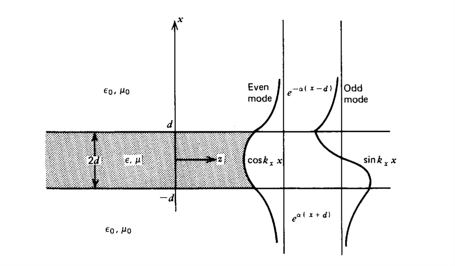
where we choose to write the solution outside the dielectric in the decaying wave form so that the fields are predominantly localized around the dielectric.

The wavenumbers and decay rate obey the relations

\[ k_{x}^{2}+k_{z}^{2}=\omega^{2}\varepsilon\mu\\
-\alpha ^{2}+k_{z}^{2}=\omega^{2}\varepsilon_{0}\mu _{0} \]

The \(z\) component of the wavenumber must be the same in all regions so that the boundary conditions can be met at each interface. For propagation in the dielectric and evanescence in free space, we must have that

\[ \omega^{2}\varepsilon_{0}\mu _{0}< k_{z}< \omega^{2}\varepsilon\mu \]

All the other electric and magnetic field components can be found from (1) in the same fashion as for metal waveguides in Section 8-6-2. However, it is convenient to separately consider each of the solutions for \(E_{z}\) within the dielectric.

(a) Odd Solutions

If \(E_{z}\) in each half-plane above and below the centerline are oppositely directed, the field within the dielectric must vary solely as \(k_{x}x\):

\[ \begin{align} \hat{E}_{z}= \left\{\begin{array}{ll}
A_{2}e^{-\alpha \left ( x-d \right )}, &\quad x\geq d\\ 
A_{1}\sin k_{x}x, &\quad \left | x \right |\leq d\\ 
A_{3}e^{\alpha \left ( x+d \right )}, & \quad x\leq -d
\end{array}\right.\end{align} \]

Then because in the absence of volume charge the electric field has no divergence,

\[ \begin{align}\frac{\partial \hat{E}_{x}}{\partial x}-jk_{z}\hat{E}_{z}\Rightarrow \hat{E}_{x}=\left\{\begin{array}{ll}
\displaystyle -\frac{jk_{z}}{\alpha }A_{2}e^{-\alpha \left ( x-d \right )},&\quad x\geq d\\ 
\displaystyle -\frac{jk_{z}}{k_{x}}A_{1}\cos k_{x}x,&\quad \left | x \right |\leq d\\ 
\displaystyle \frac{jk_{z}}{\alpha }A_{3}e^{\alpha \left ( x+d \right )},&\quad x\leq  -d
\end{array}\right.\end{align} \]

while from Faraday's law the magnetic field is

\[ \begin{align}\hat{H}_{y}=-\frac{1}{j\omega \mu }\left ( -jk_{z}\hat{E}_{x}-\frac{\partial \hat{E}_{z}}{\partial x} \right ) \\
\Rightarrow \hat{H}_{y}=\left\{\begin{array}{ll}
\displaystyle -\frac{j\omega \varepsilon _{0}A_{2}}{\alpha }e^{-\alpha \left ( x-d \right )},&\quad x\geq d \nonumber \\ 
\displaystyle -\frac{j\omega \varepsilon A_{1}}{k_{x}}\cos k_{x}x,&\quad \left | x \right |\leq d \nonumber \\ 
\displaystyle \frac{j\omega \varepsilon _{0}A_{3}}{\alpha }e^{\alpha \left ( x+d \right )},&\quad x\leq -d
\nonumber \end{array}\right.\end{align} \]

At the boundaries where \(x=\pm d\) the tangential electric and magnetic fields are continuous:

\begin{align}E_{z}\left (x=\pm d_{-} \right )=E_{z}\left (x=\pm d_{+} \right )\Rightarrow &A_{1}\sin k_{x}d=A_{2} \\ &
-A_{1}\sin k_{x}d=A_{3} \nonumber \\
H_{y}\left (x=\pm d_{-} \right )=H_{y}\left (x=\pm d_{+} \right )\Rightarrow &\frac{-j\omega \varepsilon A_{1}}{k_{x}}\cos k_{x}d=\frac{-j\omega \varepsilon_{0} A_{2}}{\alpha } \nonumber \\ &
\frac{-j\omega \varepsilon A_{1}}{k_{x}}\cos k_{x}d=\frac{j\omega \varepsilon_{0} A_{3}}{\alpha } \nonumber \end{align}

which when simultaneously solved yields

\[\]\[ \left.\begin{matrix}
\displaystyle\frac{A_{2}}{A_{1}}=\sin k_{x}d=\frac{\varepsilon \alpha }{\varepsilon _{0}k_{x}}\cos k_{x}d\\ 
\displaystyle\frac{A_{3}}{A_{1}}=-\sin k_{x}d=-\frac{\varepsilon \alpha }{\varepsilon _{0}k_{x}}\cos k_{x}d
\end{matrix}\right\}\Rightarrow \alpha =\frac{\varepsilon _{0}}{\varepsilon }k_{x}\tan k_{x}d \nonumber \]

The allowed values of \(\alpha\) and \(k_{x}\) are obtained by self-consistently solving (8) and (2), which in general requires a numerical method. The critical condition for a guided wave occurs when \(\alpha =0\), which requires that \(k_{x}d=n\pi \) and \(k_{z}^{2}=\omega ^{2}\varepsilon _{0}\mu _{0}\). The critical frequency is then obtained from (2) as

\[ \omega ^{2}=\frac{k_{x}^{2}}{\varepsilon \mu -\varepsilon _{0}\mu _{0} }=\frac{\left ( n\pi /d \right )^{2}}{\varepsilon \mu -\varepsilon _{0}\mu _{0} } \]

Note that this occurs for real frequencies only if \(\varepsilon \mu > \varepsilon _{0}\mu _{0} \).

(b) Even Solutions

If \(E_{z}\) is in the same direction above and below the dielectric, solutions are similarly

\begin{align} \hat{E}_{z}= \left\{\begin{array}{ll}
B_{2}e^{-\alpha \left ( x-d \right )}, &\quad x\geq d\\ 
B_{1}\cos  k_{x}x, &\quad \left | x \right |\leq d \nonumber \\ 
B_{3}e^{\alpha \left ( x+d \right )}, & \quad x\leq -d
\nonumber \end{array}\right.\end{align}

\begin{align}\hat{E}_{x}=\left\{\begin{array}{ll}
\displaystyle -\frac{jk_{z}}{\alpha }B_{2}e^{-\alpha \left ( x-d \right )},&\quad x\geq d\\ 
\displaystyle \frac{jk_{z}}{k_{x}}B_{1}\sin k_{x}x,&\quad \left | x \right |\leq d \nonumber \\ 
\displaystyle \frac{jk_{z}}{\alpha }B_{3}e^{\alpha \left ( x+d \right )},&\quad x\leq  -d
\nonumber \end{array}\right.\end{align}

\begin{align}\hat{H}_{y}=\left\{\begin{array}{ll}
\displaystyle -\frac{j\omega \varepsilon _{0}}{\alpha }B_{2}e^{-\alpha \left ( x-d \right )},&\quad x\geq d\\ 
\displaystyle \frac{j\omega \varepsilon }{k_{x}}B_{1}\sin k_{x}x,&\quad \left | x \right |\leq d \nonumber \\ 
\displaystyle \frac{j\omega \varepsilon _{0}}{\alpha }B_{3}e^{\alpha \left ( x+d \right )},&\quad x\leq -d
\nonumber \end{array}\right.\end{align}

Continuity of tangential electric and magnetic fields at \(x=\pm d\) requires

\[ B_{1}\cos k_{x}d=B_{2},\quad B_{1}\cos k_{x}d=B_{3}\\
\frac{j\omega \varepsilon }{k_{x}}B_{1}\sin k_{x}d=-\frac{j\omega \varepsilon _{0}}{\alpha }B_{2},\quad 
-\frac{j\omega \varepsilon B_{1}}{k_{x}}\sin k_{x}d=\frac{j\omega \varepsilon _{0}B_{3}}{\alpha } \]

or

\[ \left.\begin{matrix}
\displaystyle \frac{B_{2}}{B_{1}}=\cos k_{x}d=-\frac{\varepsilon \alpha }{\varepsilon _{0}k_{x}}\sin k_{x}d\\ 
\displaystyle \frac{B_{3}}{B_{1}}=\cos k_{x}d=-\frac{\varepsilon \alpha }{\varepsilon _{0}k_{x}}\sin k_{x}d
\end{matrix}\right\} \Rightarrow \alpha =-\frac{\varepsilon _{0}k_{x}}{\varepsilon }\cot k_{x}d \]

TE Solutions

The same procedure is performed for the \(\textrm{TE}\) solutions by first solving for \(H_{z}\).

(a) Odd Solutions

\begin{align} \hat{H}_{z}= \left\{\begin{array}{ll}
A_{2}e^{-\alpha \left ( x-d \right )}, &\quad x\geq d\\ 
A_{1}\sin k_{x}x, &\quad \left | x \right |\leq d\\ 
A_{3}e^{\alpha \left ( x+d \right )}, & \quad x\leq -d
\end{array}\right.\end{align}

\begin{align}\hat{H}_{x}=\left\{\begin{array}{ll}
\displaystyle -\frac{jk_{z}}{\alpha }A_{2}e^{-\alpha \left ( x-d \right )},&\quad x\geq d\\ 
\displaystyle -\frac{jk_{z}}{k_{x}}A_{1}\cos k_{x}x,&\quad \left | x \right |\leq d\\ 
\displaystyle \frac{jk_{z}}{\alpha }A_{3}e^{\alpha \left ( x+d \right )},&\quad x\leq  -d
\end{array}\right.\end{align}

\begin{align}
\hat{E}_{y}=\left\{\begin{array}{ll}
\displaystyle \frac{j\omega \mu _{0}}{\alpha }A_{2}e^{-\alpha \left ( x-d \right )},&\quad x\geq d\\ 
\displaystyle \frac{j\omega \mu }{k_{x}}A_{1}\cos k_{x}x,&\quad \left | x \right |\leq d\\ 
\displaystyle -\frac{j\omega\mu _{0}}{\alpha }A_{3}e^{\alpha \left ( x+d \right )},&\quad x\leq -d
\end{array}\right.\end{align} 

where continuity of tangential \(\textbf{E}\) and \(\textbf{H}\) across the boundaries requires

\[\alpha =\frac{\mu _{0}}{\mu }k_{x}\tan k_{x}d \]

(b) Even Solutions

\begin{align} \hat{H}_{z}= \left\{\begin{array}{ll}
B_{2}e^{-\alpha \left ( x-d \right )}, &\quad x\geq d\\ 
B_{1}\cos  k_{x}x, &\quad \left | x \right |\leq d\\ 
B_{3}e^{\alpha \left ( x+d \right )}, & \quad x\leq -d
\end{array}\right.\end{align}

\begin{align}\hat{H}_{x}=\left\{\begin{array}{ll}
\displaystyle -\frac{jk_{z}}{\alpha }B_{2}e^{-\alpha \left ( x-d \right )},&\quad x\geq d\\ 
\displaystyle \frac{jk_{z}}{k_{x}}B_{1}\sin k_{x}x,&\quad \left | x \right |\leq d\\ 
\displaystyle \frac{jk_{z}}{\alpha }B_{3}e^{\alpha \left ( x+d \right )},&\quad x\leq  -d
\end{array}\right.\end{align}

\begin{align}\hat{E}_{y}=\left\{\begin{array}{ll}
\displaystyle \frac{j\omega \mu  _{0}}{\alpha }B_{2}e^{-\alpha \left ( x-d \right )},&\quad x\geq d\\ 
\displaystyle -\frac{j\omega \mu }{k_{x}}B_{1}\sin k_{x}x,&\quad \left | x \right |\leq d\\ 
\displaystyle -\frac{j\omega \mu_{0}}{\alpha }B_{3}e^{\alpha \left ( x+d \right )},&\quad x\leq -d
\end{array}\right.\end{align}

where \(\alpha\) and \(k_{x}\) are related as

\[ \alpha =-\frac{\mu _{0}}{\mu }k_{x}\cot k_{x}d \]