
8.8: Problems
- Page ID
- 83360

Section 8-1
Find the inductance and capacitance per unit length and the characteristic impedance for the wire above plane and two wire line shown in Figure 8-3. (Hint: See Section 2-6-4c.)
The inductance and capacitance per unit length on a lossless transmission line is a weak function of \(z\) as the distance between electrodes changes slowly with \(z\).
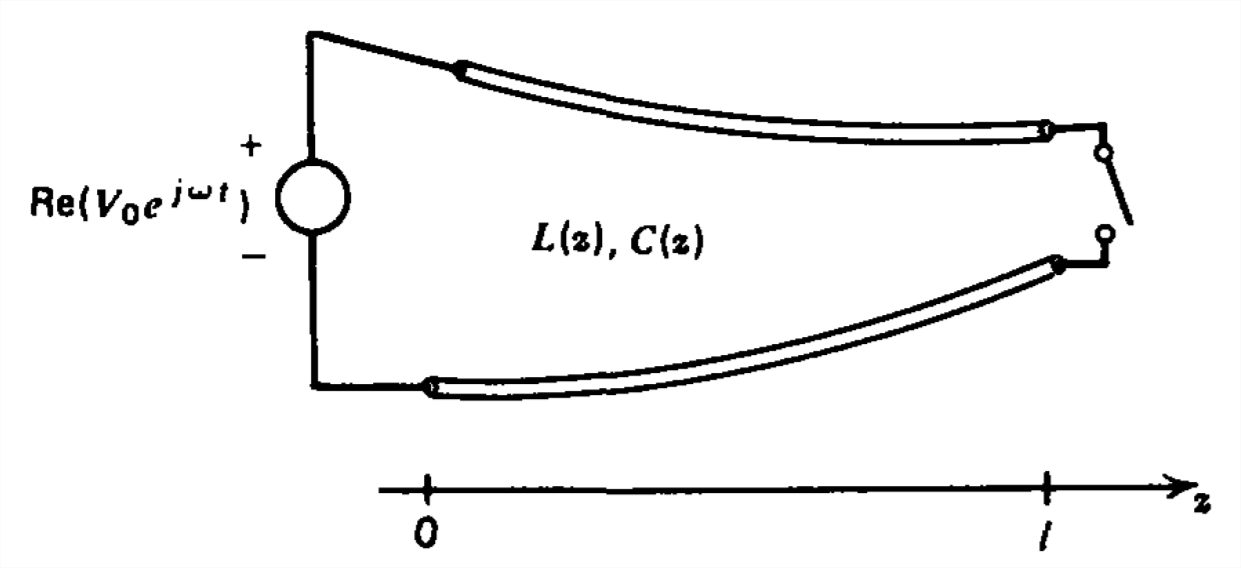
(a) For this case write the transmission line equations as single equations in voltage and current.
(b) Consider an exponential line, where
\(L\left ( z \right )=L_{0}e^{\alpha z},\quad C\left ( z \right )=C_{0}e^{-\alpha z}\)
If the voltage and current vary sinusoidally with time as
\(v\left ( z,t \right )=\textrm{Re}\left [ \hat{v}\left ( z \right )e^{j\omega t} \right ],\quad i\left ( z,t \right )=\textrm{Re}\left [ \hat{\pmb{\imath}}\left ( z \right )e^{j\omega t} \right ]\)
find the general form of solution for the spatial distributions of \(\hat{v}\left ( z \right )\) and \(\hat{\pmb{\imath}}\left ( z \right )\).
(c) The transmission line is excited by a voltage source \(V_{0}\cos \omega t\) at \(z=0\). What are the voltage and current distributions if the line is short or open circuited at \(z=l\)?
(d) For what range of frequency do the waves strictly decay with distance? What is the cut-off frequency for wave propagation?
(e) What are the resonant frequencies of the short circuited line?
(f) What condition determines the resonant frequencies of the open circuited line.
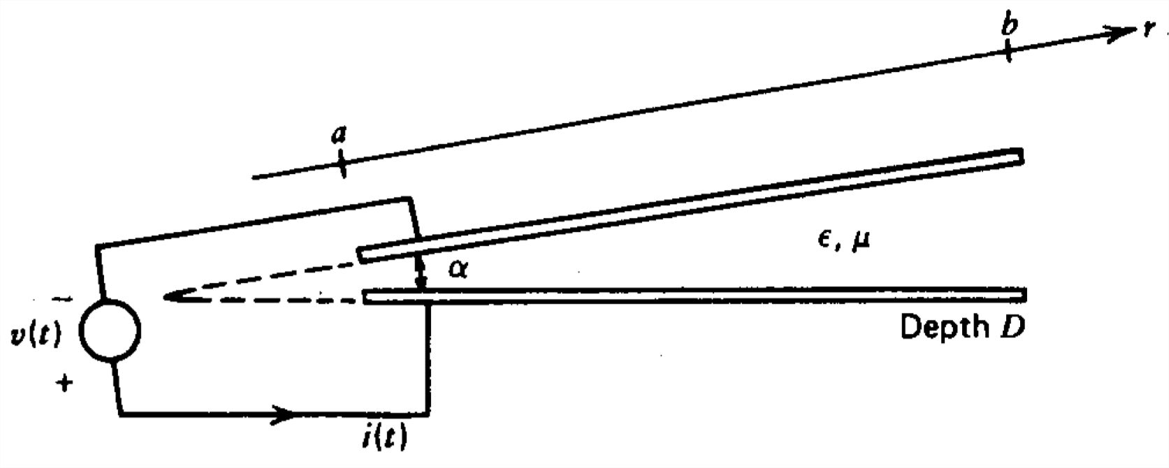
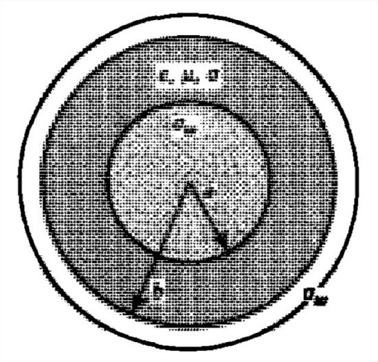
Two conductors of length \(l\) extending over the radial distance \(a\leq \textrm{r}\leq b\) are at a constant angle \(\alpha \) apart.
(a) What are the electric and magnetic fields in terms of the voltage and current?
(b) Find the inductance and capacitance per unit length. What is the characteristic impedance?
A parallel plate transmission line is filled with a conducting plasma with constitutive law
\(\frac{\partial \textbf{J}}{\partial t}=\omega_{p}^{2}\varepsilon \textbf{E}\)
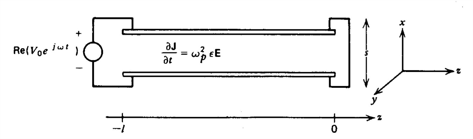
(a) How are the electric and magnetic fields related?
(b) What are the transmission line equations for the voltage and current?
(c) For sinusoidal signals of the form \(e^{j\left ( \omega t-kz \right )}\), how are \(\omega\) and \(k\) related? Over what frequency range do we have propagation or decay?
(d) The transmission line is short circuited at \(z = 0\) and excited by a voltage source \(V_{0}\cos \omega t\) at \(z=-l\). What are the voltage and current distributions?
(e) What are the resonant frequencies of the system?
An unusual type of distributed system is formed by series capacitors and shunt inductors.
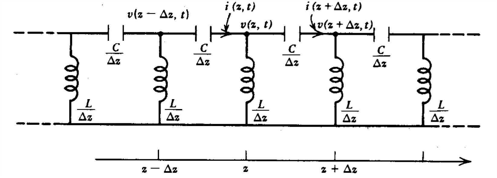
(a) What are the governing partial differential equations relating the voltage and current?
(b) What is the dispersion relation between \(\omega \) and \(k\) for signals of the form \(e^{j\left ( \omega t-kz \right )}\)?
(c) What are the group and phase velocities of the waves? Why are such systems called "backward wave"?
(d) A voltage \(V_{0}\cos \omega t\) is applied at \(z=-l\) with the \(z= 0\) end short circuited. What are the voltage and current distributions along the line?
(e) What are the resonant frequencies of the system?
Section 8-2
An infinitely long transmission line is excited at its center by a step voltage \(V_{0}\) turned on at \(t=0\). The line is initially at rest.
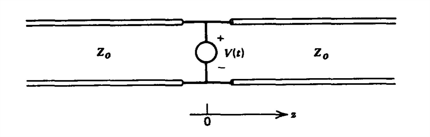
(a) Plot the voltage and current distributions at time \(T\).
(b) At this time \(T\) the voltage is set to zero. Plot the voltage and current everywhere at time \(2T\).
A transmission line of length \(l\) excited by a step voltage source has its ends connected together. Plot the voltage and current at \(z=l/4\), \(l/2\) and \(3l/4\) as a function of time.
The dc steady state is reached for a transmission line loaded at \(z=l\) with a resistor \(R_L\) and excited at \(z=0\) by a dc voltage \(V_{0}\) applied through a source resistor \(R_s\). The voltage source is suddenly set to zero at \(t=0\).
(a) What is the initial voltage and current along the line?
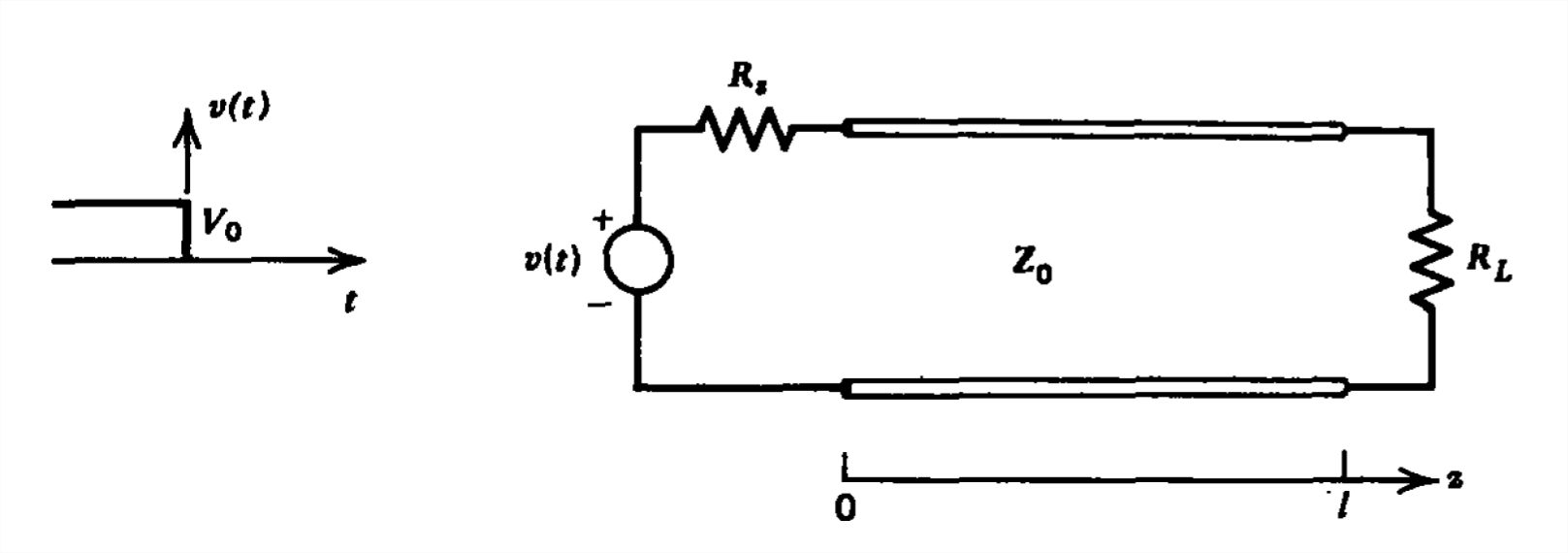
(b) Find the voltage at the \(z=l\) end as a function of time. (Hint: Use difference equations.)
A step current source turned on at \(t = 0\) is connected to the \(z=0\) end of a transmission line in parallel with a source resistance \(R_s\). A load resistor \(R_L\) is connected at \(z=l\).
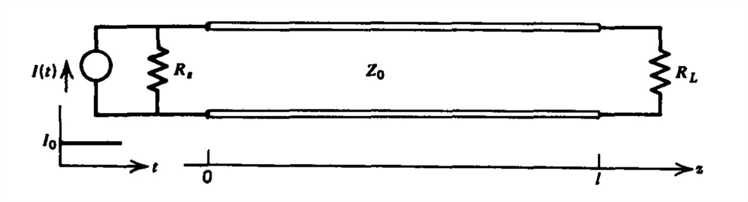
(a) What is the load voltage and current as a function of time? (Hint: Use a Thevenin equivalent network at \(z =0\) with the results of Section 8-2-3.)
(b) With \(R_s=\infty \) plot versus time the load voltage when \(R_L=\infty \) and the load current when \(R_L=0\).
(c) If \(R_s=\infty \) and \(R_L=\infty \), solve for the load voltage in the quasi-static limit assuming the transmission line is a capacitor. Compare with (b).
(d) If \(R_s\) is finite but \(R_L=0\), what is the time dependence of the load current?
(e) Repeat (d) in the quasi-static limit where the trans mission line behaves as an inductor. When are the results of (d) and (e) approximately equal?
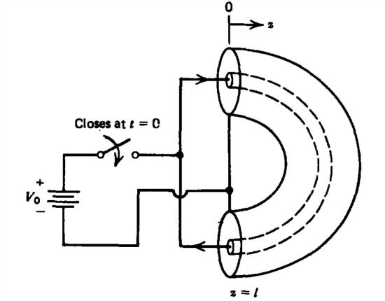
Switched transmission line systems with an initial dc voltage can be used to generate high voltage pulses of short time duration. The line shown is charged up to a dc voltage \(V_{0}\) when at \(t =0\) the load switch is closed and the source switch is opened.
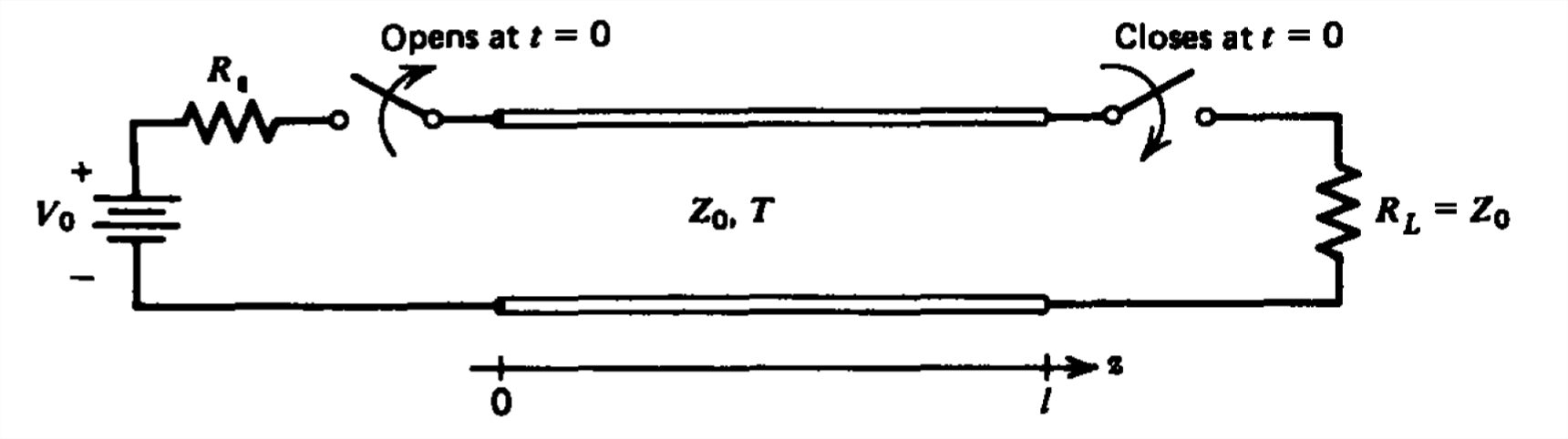
(a) What are the initial line voltage and current? What are \(V_{+}\) and \(V_{-}\)?
(b) Sketch the time dependence of the load voltage.
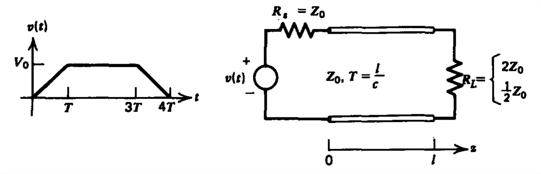
For the trapezoidal voltage excitation shown, plot versus time the current waveforms at \(z =0\) and \(z=l\) for \(R_{L}=2Z_{0}\) and \(R_{L}=\frac{1}{2}Z_{0}\).
A step voltage is applied to a loaded transmission line with \(R_{L}=2Z_{0}\) through a matching source resistor.
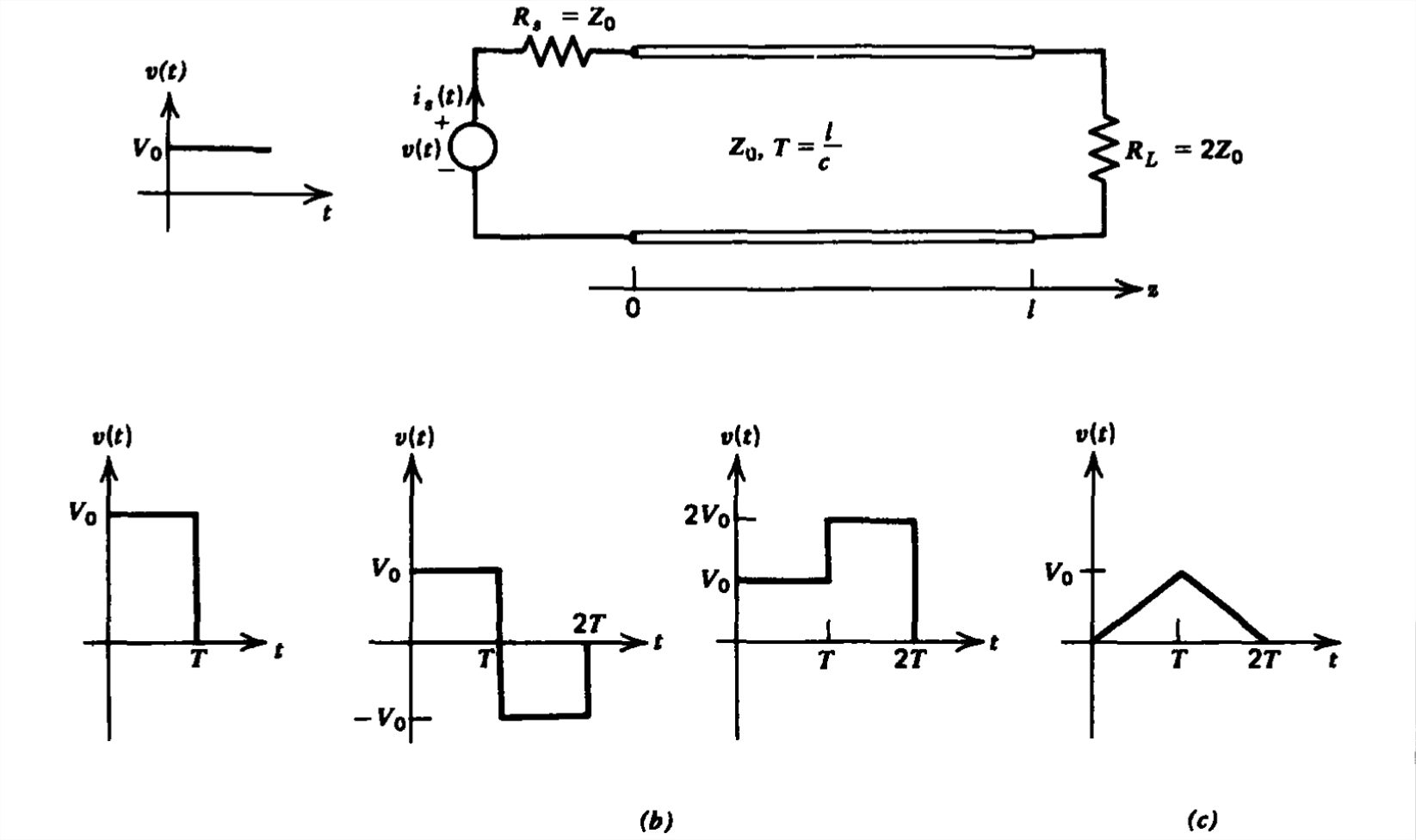
(a) Sketch the source current \(i_{s}\left ( t \right )\).
(b) Using superposition of delayed step voltages find the time dependence of \(i_{s}\left ( t \right )\) for the various pulse voltages shown.
(c) By integrating the appropriate solution of (b), find \(i_{s}\left ( t \right )\) if the applied voltage is the triangle wave shown.
A dc voltage has been applied for a long time to the .transmission line circuit shown with switches \(S_{1}\) and\(S_{2}\) open when at \(t=0\):
(a) \(S_{2}\) is suddenly closed with \(S_{1}\) kept open;
(b) \(S_{1}\) is suddenly closed with \(S_{2}\) kept open;
(c) Both \(S_{1}\) and \(S_{2}\) are closed.
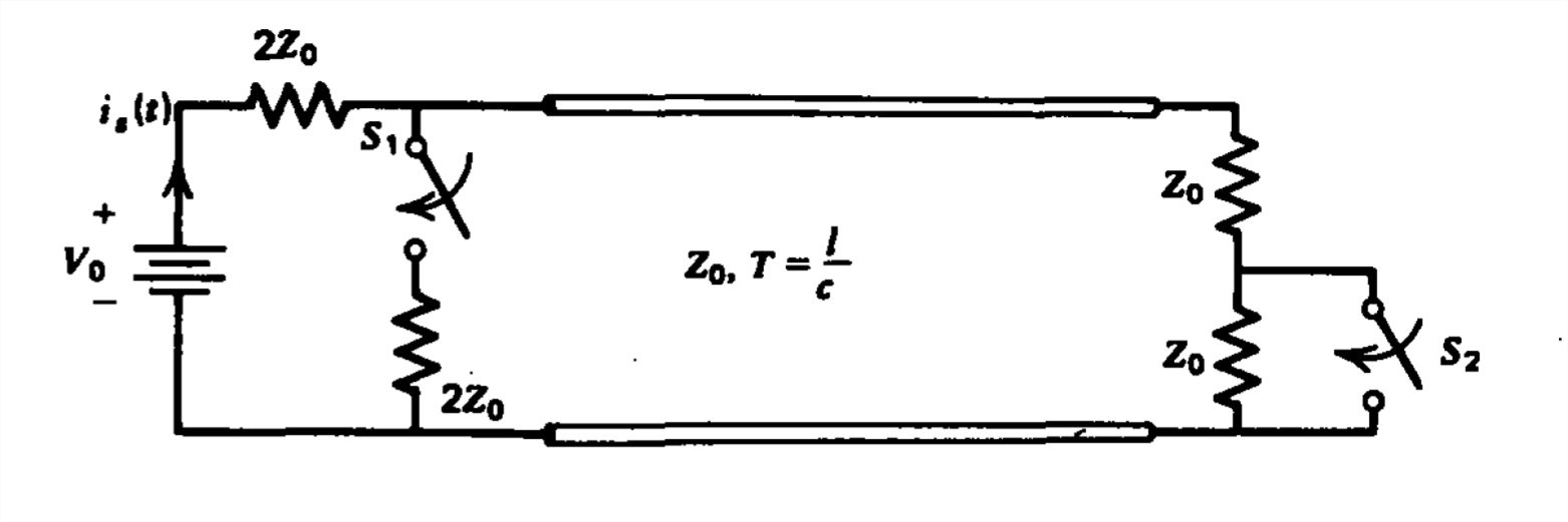
For each of these cases plot the source current \(i_{s}\left ( t \right )\) versus time.
For each of the transmission line circuits shown, the switch opens at \(t=0\) after the dc voltage has been applied for a long time.
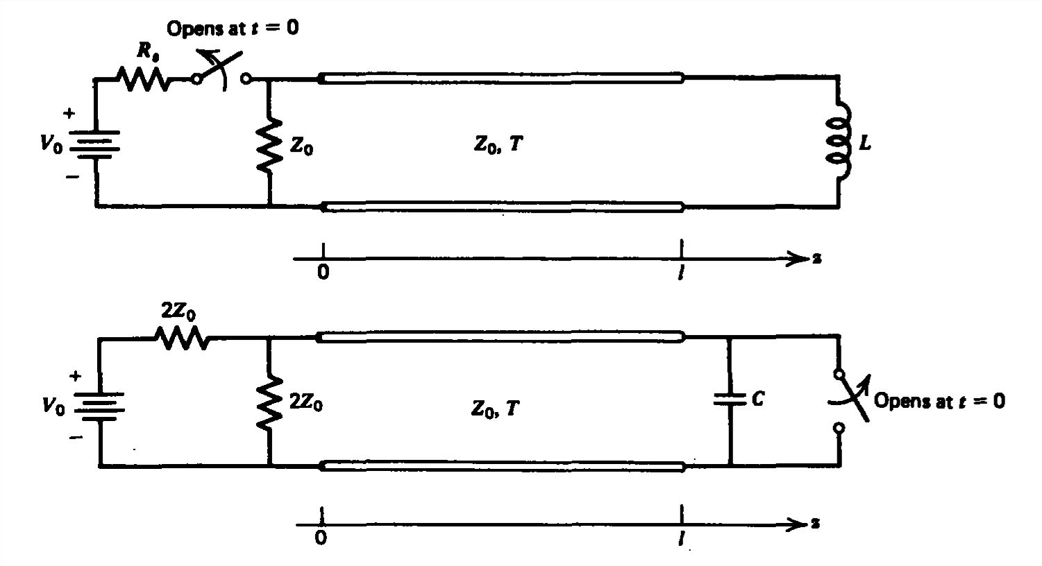
(a) What are the transmission line voltages and currents right before the switches open? What are \(V_{+}\) and \(V_{-}\) at \(t=0\)?
(b) Plot the voltage and current as a function of time at
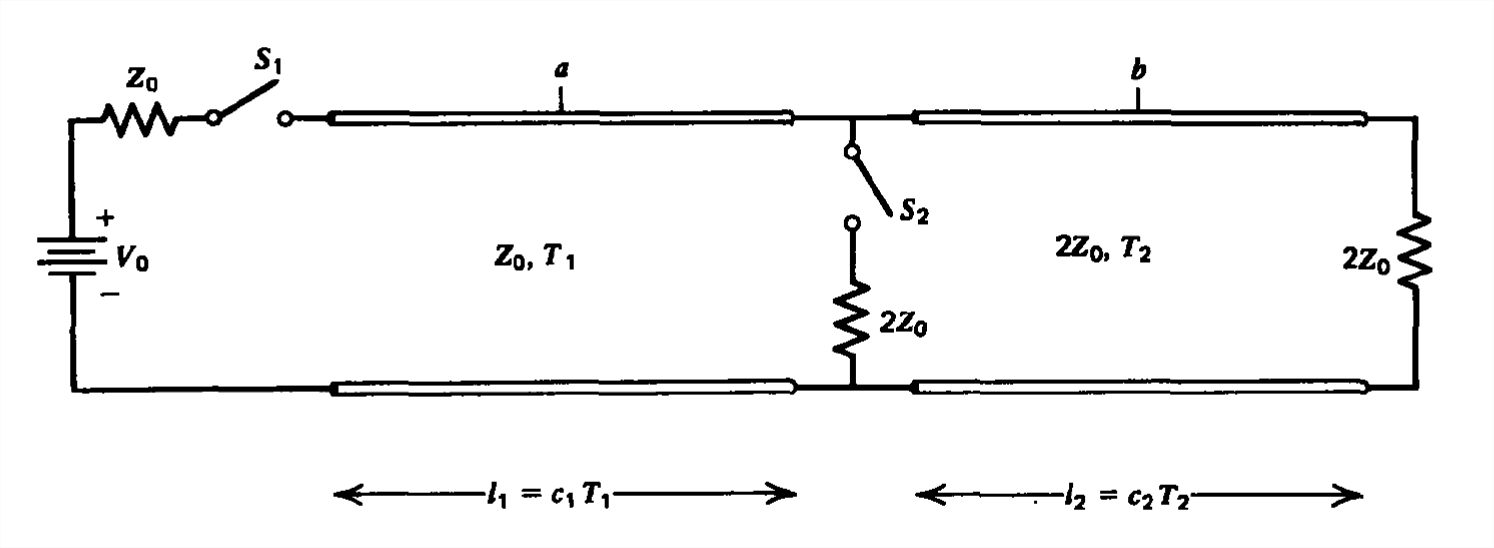
A transmission line is connected to another transmission line with double the characteristic impedance.
(a) With switch \(S_{2}\) open, switch \(S_{1}\) is suddenly closed at \(t=0\). Plot the voltage and current as a function of time half way down each line at points \(a\) and \(b\).
(b) Repeat (a) if \(S_{2}\) is closed.
Section 8-3
A transmission line is excited by a voltage source \(V_{0}\cos \omega t\) at \(z=-l\). The transmission line is loaded with a purely reactive load with impedance \(jX\) at \(z =0\).
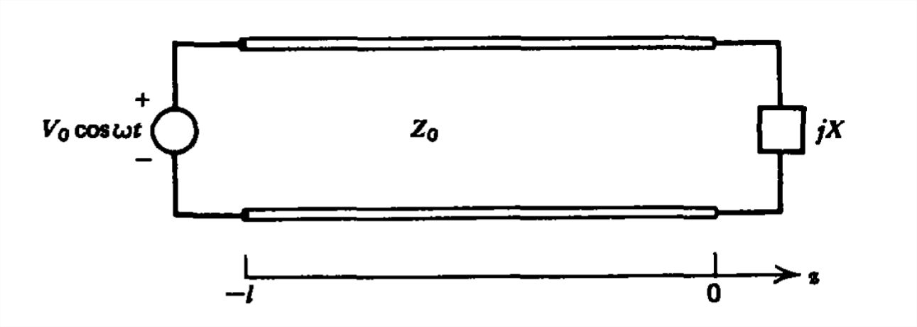
(a) Find the voltage and current distribution along the line.
(b) Find an expression for the resonant frequencies of the system if the load is capacitive or inductive. What is the solution if \(\left | X \right |=Z_{0}\)?
(c) Repeat (a) and (b) if the transmission line is excited by a current source \(I_{0}\cos \omega t\) at \(z=-l\).
(a) Find the resistance and conductance per unit lengths for a coaxial cable whose dielectric has a small Ohmic conductivity \(\sigma \) and walls have a large conductivity \(\sigma _{w}\), (Hint: The skin depth \(\delta \) is much smaller than the radii or thickness of either conductor.)
(b) What is the decay rate of the fields due to the losses?
(c) If the dielectric is lossless \(\left ( \sigma =0 \right )\) with a fixed value of outer radius \(b\), what value of inner radius \(a\) will minimize the decay rate? (Hint: \(1+1/3.6\approx \textrm{ln}\,3.6\).)
A transmission line of length \(l\) is loaded by a resistor \(R_{L}\).
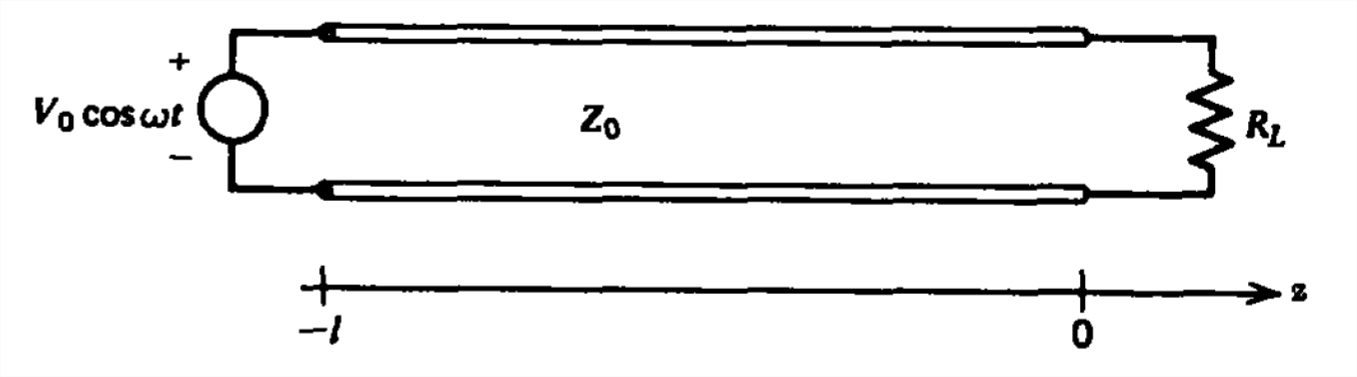
(a) Find the voltage and current distributions along the line.
(b) Reduce the solutions of (a) when the line is much shorter than a wavelength.
(c) Find the approximate equivalent circuits in the long wavelength limit \(\left ( kl\ll 1 \right )\) when \(R_{L}\) is very small \(\left ( R_{L}\ll Z_{0} \right )\) and when it is very large \(\left ( R_{L}\gg Z_{0} \right )\).
Section 8-4
For the transmission line shown:
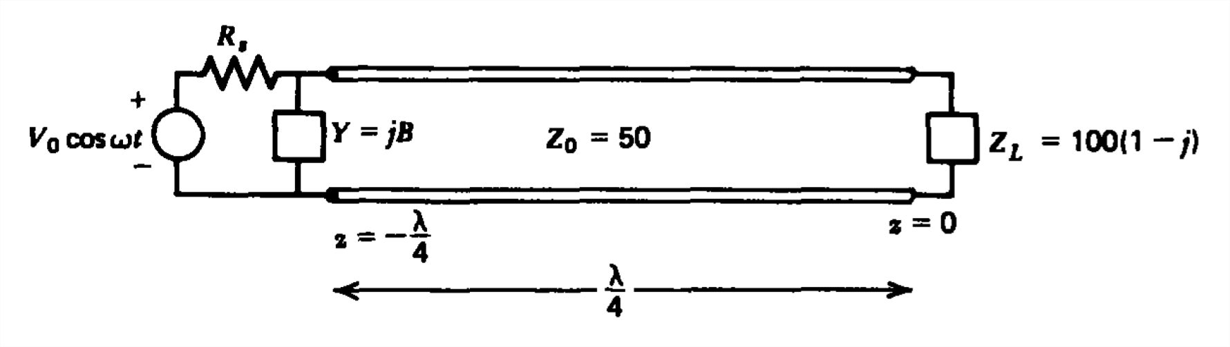
(a) Find the values of lumped reactive admittance \(Y=jB\) and non-zero source resistance \(R_{s}\) that maximizes the power delivered by the source. (Hint: Do not use the Smith chart.)
(b) What is the time-average power dissipated in the load?
(a) Find the time-average power delivered by the source for the transmission line system shown when the switch is open or closed. (Hint: Do not use the Smith chart.)
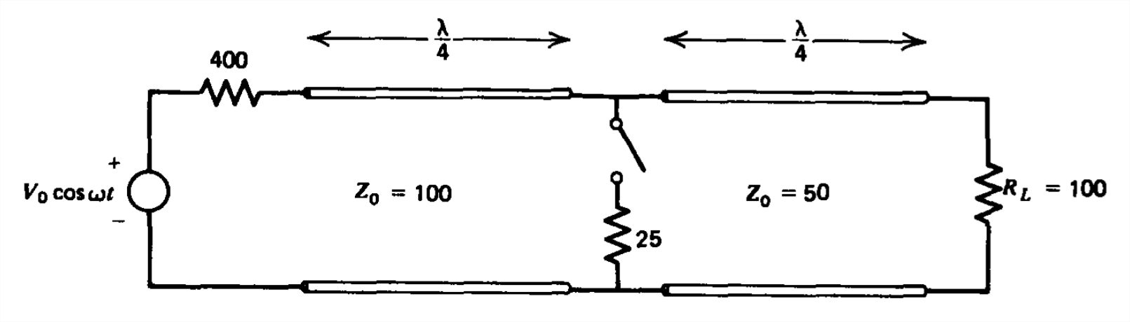
(b) For each switch position, what is the time average power dissipated in the load resistor \(R_{L}\)?
(c) For each switch position what is the \(\textrm{VSWR}\) on each line?
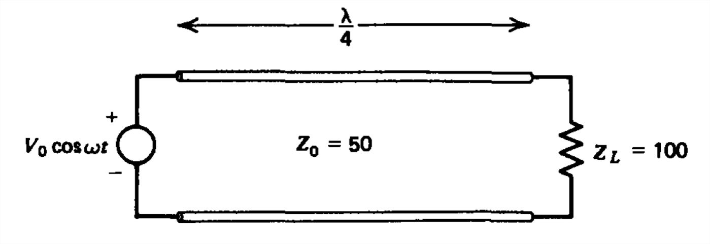
(a) Using the Smith chart find the source current delivered (magnitude and phase) for the transmission line system shown, for \(l=\lambda /8\), \(\lambda /4\), \(3\lambda /8\), and \(\lambda /2\).
(b) For each value of \(l\), what are the time-average powers delivered by the source and dissipated in the load impedance \(Z_{L}\)?
(c) What is the \(\textrm{VSWR}\)?
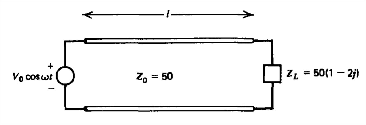
(a) Without using the Smith chart find the voltage and current distributions for the transmission line system shown.
(b) What is the \(\textrm{VSWR}\)?
(c) At what positions are the voltages a maximum or a minimum? What is the voltage magnitude at these positions?
The \(\textrm{VSWR}\) on a \(100 \textrm{Ohm}\) transmission line is \(3\). The distance between successive voltage minima is \(50\,\textrm{cm}\) while the distance from the load to the first minima is \(20\,\textrm{cm}\). What are the reflection coefficient and load impedance?
Section 8-5
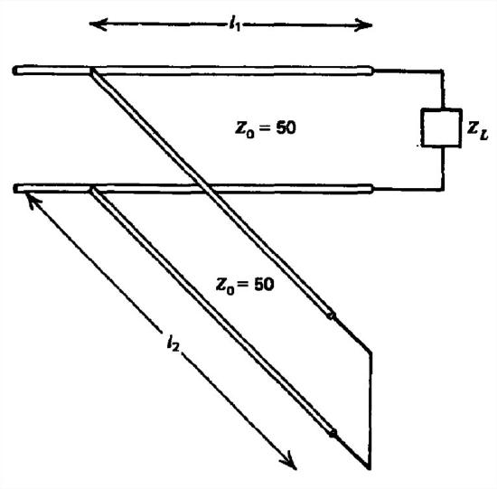
For each of the following load impedances in the single-stub tuning transmission line system shown, find all values of the length of the line \(l_1\) and stub length \(l_2\) necessary to match the load to the line.
(a) \(Z_L=100\left ( 1-j \right )\) (c) \(Z_L=25\left ( 2-j \right )\)
(b) \(Z_L=50\left ( 1+2j \right )\) (d) \(Z_L=25\left ( 1+2j \right )\)
For each of the following load impedances in the double-stub tuning transmission line system shown, find stub lengths \(l_1\) and \(l_2\) to match the load to the line.
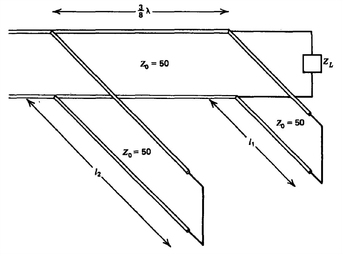
(a) \(Z_L=100\left ( 1-j \right )\) (c) \(Z_L=25\left ( 2-j \right )\)
(b) \(Z_L=50\left ( 1+2j \right )\) (d) \(Z_L=25\left ( 1+2j \right )\)
(a) Without using the Smith chart, find the input impedance \(Z_{in}\) at \(z=-l=-\lambda /4\) for each of the loads shown.
(b) What is the input current \(i\left ( z=-l,t \right )\) for each of the loads?
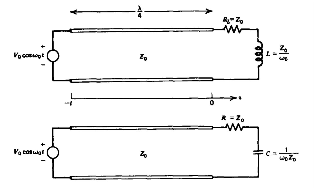
(c) The frequency of the source is doubled to \(2\omega _{0}\). The line length \(l\) and loads \(L\) and \(C\) remain unchanged. Repeat (a) and (b).
(d) The frequency of the source is halved to \(\frac{1}{2}\omega _{0}\). Repeat (a) and (b).
Section 8-6
A rectangular metal waveguide is filled with a plasma with constitutive law
\(\frac{\partial \textbf{J}_{f}}{\partial \textbf{t}}=\omega _{p}^{2}\varepsilon \textbf{E}\)
(a) Find the \(\textrm{TE}\) and \(\textrm{TM}\) solutions that satisfy the boundary conditions.
(b) What is the wavenumber \(k_z\) along the axis? What is the cut-off frequency?
(c) What are the phase and group velocities of the waves?
(d) What is the total electromagnetic power flowing down the waveguide for each of the modes?
(e) If the walls have a large but finite conductivity, what is the spatial decay rate for \(\textrm{TE}_{10}\) propagating waves?
(a) Find the power dissipated in the walls of a waveguide with large but finite conductivity \(\sigma _{w}\) for the \(\textrm{TM}_{mn}\) modes (Hint: Use Equation (25).)
(b) What is the spatial decay rate for propagating waves?
(a) Find the equations of the electric and magnetic field lines in the \(xy\) plane for the \(\textrm{TE}\) and \(\textrm{TM}\) modes.
(b) Find the surface current field lines on each of the waveguide surfaces for the \(\textrm{TM}_{mn}\) modes. Hint:
\(\int \tan xdx=-\ln \cos x\)
\(\int \cot xdx=\ln \sin x\)
(c) For all modes verify the conservation of charge relation on the \(x = 0\) surface:
\(\nabla _{\sum }\cdot \textbf{K}+\frac{\partial \sigma _{f}}{\partial t}=0\)
(a) Find the first ten lowest cut-off frequencies if \(a=b=1\,\textrm{cm}\) in a free space waveguide.
(b) What are the necessary dimensions for a square free space waveguide to have a lowest cut-off frequency of \(10^{10}\), \(10^{8}\), \(10^{6}\), \(10^{4}\), or \(10^{2}\)?
A rectangular waveguide of height \(b\) and width \(a\) is short circuited by perfectly conducting planes at \(z=0\) and \(z=l\).
(a) Find the general form of the \(\textrm{TE}\) and \(\textrm{TM}\) electric and magnetic fields. (Hint: Remember to consider waves travel ing in the \(\pm z\) directions.)
(b) What are the natural frequencies of this resonator?
(c) If the walls have a large conductivity \(\sigma _{w}\) find the total time-average power \(<P_d>\) dissipated in the \(\textrm{TE}_{101}\) mode.
(d) What is the total time-average electromagnetic energy \(<W>\) stored in the resonator?
(e) Find the \(\mathcal{Q}\) of the resonator, defined as
\(\mathcal{Q}=\frac{\omega _0<W>}{<P_{d}>}\)
where \(\omega _0\) is the resonant frequency.
Section 8.7
(a) Find the critical frequency where the spatial decay rate \(\alpha \) is zero for all the dielectric modes considered.
(b) Find approximate values of \(\alpha \), \(k_{x}\), and \(k_{z}\) for a very thin dielectric, where \(k_{x}d\ll 1\).
(c) For each of the solutions find the time-average power per unit length in each region.
(d) If the dielectric has a small Ohmic conductivity \(\sigma \), what is the approximate attenuation rate of the fields.
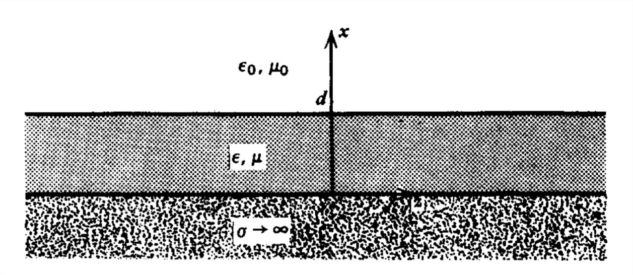
A dielectric waveguide of thickness \(d\) is placed upon a perfect conductor.
(a) Which modes can propagate along the dielectric?
(b) For each of these modes, what are the surface current and charges on the conductor?
(c) Verify the conservation of charge relation:
\(\nabla _{\sum }\cdot \textbf{K}+\frac{\partial \sigma _{f}}{\partial t}=0\)
(d) If the conductor has a large but noninfinite Ohmic conductivity \(\sigma _{w}\), what is the approximate power per unit area dissipated?
(e) What is the approximate attenuation rate of the fields?