9.2: Radiation from Point Dipole

The Electric Dipole

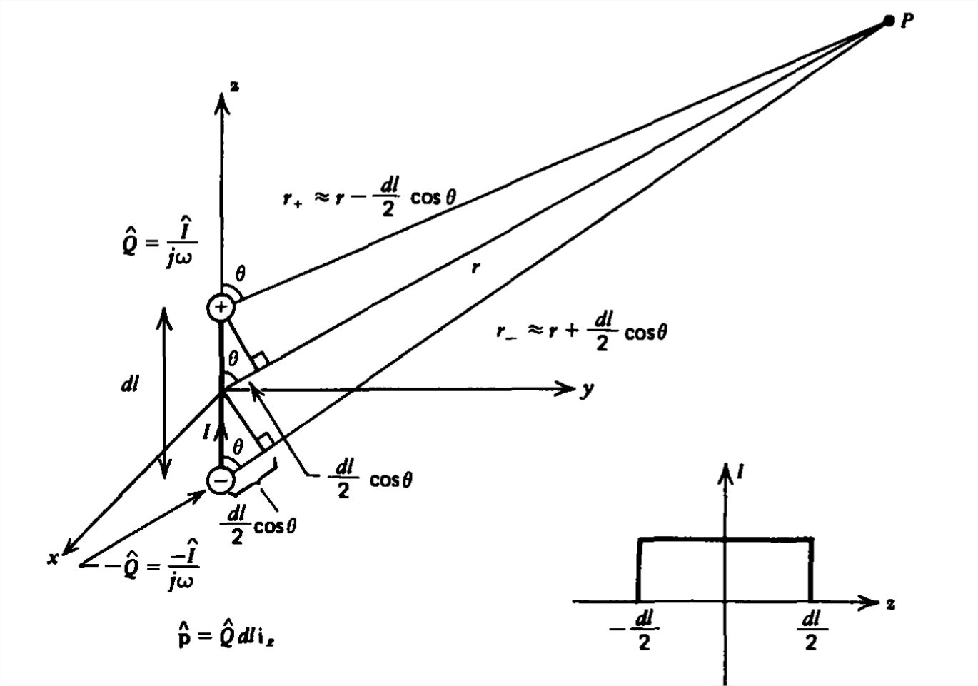
The simplest building block for a transmitting antenna is that of a uniform current flowing along a conductor of incremental length \(\)dl as shown in Figure 9-1. We assume that this current varies sinusoidally with time as

\[  i\left ( t \right )=\textrm{Re}\left ( \hat{I}e^{j\omega t} \right ) \]

Because the current is discontinuous at the ends, charge must be deposited there being of opposite sign at each end \(\left [ q\left ( t \right )=\textrm{Re}\left ( \hat{\mathcal{Q}}e^{j\omega t} \right ) \right ]\):

\[ i\left ( t \right )=\pm \frac{dq}{dt}\Rightarrow \hat{I}=\pm j\omega \hat{\mathcal{Q}},\quad z=\pm \frac{dl}{2} \]

This forms an electric dipole with moment

\[ \textbf{p}=q\,dl\,\textbf{i}_{z} \]

If we can find the potentials and fields from this simple element, the solution for any current distribution is easily found by superposition.

Figure 9-1 A point dipole antenna is composed of a very short uniformly distributed current-carrying wire. Because the current is discontinuous at the ends, equal magnitude but opposite polarity charges accumulate there forming an electric dipole.

By symmetry, the vector potential cannot depend on the angle \(\phi \),

\[ A_{z}=\textbf{Re}\left [ \hat{A}_{z}\left ( r,\theta  \right )e^{j\omega t} \right ] \]

and must be in the same direction as the current:

\[ A_{z}\left ( r,t \right )=\textrm{Re}\left [ \int_{-dl/2}^{+dl/2}\frac{\mu \hat{I}e^{j\left [ \omega \left ( t-r_{\mathcal{Q}P}/c \right ) \right ]}}{4\pi r_{\mathcal{Q}P}} dz \right ] \]

Because the dipole is of infinitesimal length, the distance from the dipole to any field point is just the spherical radial distance \(r\) and is constant for all points on the short wire. Then the integral in (5) reduces to a pure multiplication to yield

\[ \hat{A}_{z}=\frac{\mu \hat{I}dl}{4\pi r}e^{-jkr},\quad A_{z}\left ( r,t \right )=\textrm{Re}\left [ \hat{A}_{z}\left ( r \right )e^{j\omega t} \right ] \]

where we again introduce the wavenumber \(k=\omega /c\) and neglect writing the sinusoidal time dependence present in all field and source quantities. The spherical components of \(\hat{A}_{z}\), are \(\left ( \textbf{i}_{z}= \textbf{i}_{r}\cos \theta -\textbf{i}_{\theta }\sin \theta  \right )\):

\[ \hat{A}_{r}=\hat{A}_{z}\cos \theta ,\quad \hat{A}_{\theta}=-\hat{A}_{z}\sin\theta ,\quad  \hat{A}_{\phi }=0 \]

Once the vector potential is known, the electric and magnetic fields are most easily found from

\[ \hat{\textbf{H}}=\frac{1}{\mu }\nabla \times \hat{\textbf{A}},\quad \textbf{H}\left ( r,t \right )=\textrm{Re}\left [ \hat{\textbf{H}}\left ( r,\theta  \right )e^{j\omega t} \right ]\\
\hat{\textbf{E}}=\frac{1}{j\omega \varepsilon }\nabla \times \hat{\textbf{H}},\quad \textbf{E}\left ( r,t \right )=\textrm{Re}\left [ \hat{\textbf{E}}\left ( r,\theta  \right )e^{j\omega t} \right ] \]

Before we find these fields, let's examine an alternate approach.

Alternate Derivation Using the Scalar Potential

It was easiest to find the vector potential for the point electric dipole because the integration in (5) reduced to a simple multiplication. The scalar potential is due solely to the opposite point charges at each end of the dipole,

\[ \hat{V}=\frac{\mathcal{Q}}{4\pi \varepsilon }\left ( \frac{e^{-jkr_{+}}}{r_{+}}-\frac{e^{-jkr_{-}}}{r_{-}} \right ) \]

where \(r_{+}\) and \(r_{-}\) are the distances from the respective dipole charges to any field point, as shown in Figure 9-1. Just as we found for the quasi-static electric dipole in Section 3-1-1, we cannot let \(r_{+}\) and \(r_{-}\) equal \(r\) as a zero potential would result. As we showed in Section 3-1-1, a first-order correction must be made, where

\[ r_{+}\approx r-\frac{dl}{2}\cos \theta \\
r_{-}\approx r+\frac{dl}{2}\cos \theta  \]

so that (9) becomes

\[ \hat{V}\approx \frac{\mathcal{Q}}{4\pi \varepsilon r}e^{-jkr}\left ( \frac{e^{jk\left ( dl/2 \right )\cos \theta }}{\left ( 1-\frac{dl}{2r}\cos \theta  \right )}-\frac{e^{-jk\left ( dl/2 \right )\cos \theta }}{\left ( 1+\frac{dl}{2r}\cos \theta  \right )} \right ) \]

Because the dipole length \(dl\) is assumed much smaller than the field distance \(r\) and the wavelength, the phase factors in the exponentials are small so they and the \(1/r\) dependence in the denominators can be expanded in a first-order Taylor series to result in:

\begin{align}\lim_{k\,dl\ll 1\\dl/r\ll 1}\hat{V}&\approx \frac{\mathcal{Q}}{4\pi \varepsilon r}e^{-jkr}\left [ \left ( 1+j\frac{k\,dl}{2}\cos \theta  \right )\left ( 1+\frac{dl}{2r}\cos \theta  \right )-\left ( 1-jk\frac{dl}{2}\cos \theta  \right )\left ( 1-\frac{dl}{2r}\cos \theta  \right )\right ] \\
&=\frac{\mathcal{Q}dl}{4\pi \varepsilon r^{2}}e^{-jkr}\cos \theta \left ( 1+jkr \right ) \nonumber \end{align}

When the frequency becomes very low so that the wavenumber also becomes small, (12) reduces to the quasi-static electric dipole potential found in Section 3-1-1 with dipole moment \(\hat{p}=\hat{\mathcal{Q}}dl\). However, we see that the radiation correction terms in (12) dominate at higher frequencies (large \(k\)) far from the dipole \(\left (kr\gg 1  \right )\) so that the potential only dies off as \(1/r\) rather than the quasi-static \(1/r^{2}\). Using the relationships \(\hat{\mathcal{Q}}=\hat{I}/j\omega \) and \(c=1/\sqrt{\varepsilon \mu }\), (12) could have been obtained immediately from (6) and (7) with the Lorentz gauge condition of Eq. (13) in Section 9-1-1:

\[ \begin{align}\hat{V}=\frac{-c^{2}}{j\omega }\nabla\cdot \hat{A}&=\frac{-c^{2}}{j\omega }\left ( \frac{1}{r^{2}}\frac{\partial }{\partial r}\left ( r^{2}\hat{A}_{r} \right )+\frac{1}{r\sin \theta }\frac{\partial }{\partial \theta }\left ( \hat{A}_{\theta }\sin \theta  \right ) \right ) \nonumber \\
&=\frac{\mu \hat{I}dlc^{2}}{4\pi j\omega }\frac{\left ( 1+jkr \right )}{r^{2}}e^{-jkr}\cos \theta \nonumber \\
&=\frac{\hat{\mathcal{Q}}dl}{4\pi \varepsilon r^{2}}\left ( 1+jkr \right )e^{-jkr}\cos \theta \nonumber \end{align} \]

The Electric and Magnetic Fields

Using (6), the fields are directly found from (8) as

 \begin{align}\hat{\textbf{H}} &=\frac{1}{\mu }\times \hat{\textbf{A}} \\
&=\textbf{i}_{\phi }\frac{1}{\mu r}\left ( \frac{\partial }{\partial r}\left ( r\hat{A}_{\theta } \right ) -\frac{\partial \hat{A}_{r}}{\partial \theta }\right ) \nonumber \\
&=-\textbf{i}_{\phi }\frac{\hat{I}dl}{4\pi }k^{2}\sin \theta \left ( \frac{1}{jkr}+\frac{1}{\left (jkr  \right )^{2}} \right )e^{-jkr} \nonumber \end{align}

\begin{align}\hat{\textbf{E}} &=\frac{1}{j\omega \varepsilon}\nabla \times \hat{\textbf{H}} \\
&=\frac{1}{j\omega \varepsilon }\left ( \frac{1}{r\sin \theta }\frac{\partial }{\partial \theta }\left ( \hat{H}_{\phi }\sin \theta  \right )\textbf{i}_{r}-\frac{1}{r}\frac{\partial }{\partial r}\left ( r\hat{H}_{\phi } \right )\textbf{i}_{\theta } \right ) \nonumber \\
&=-\frac{\hat{I}dlk^{2}}{4\pi }\sqrt{\frac{\mu }{\varepsilon }}\left \{  \textbf{i}_{r}\left [ 2\cos \theta \left ( \frac{1}{\left ( jkr \right )^{2}}+\frac{1}{\left ( jkr \right )^{3}} \right ) \right ] + \textbf{i}_{\theta }\left [ \sin \theta \left ( \frac{1}{jkr}+\frac{1}{\left ( jkr \right )^{2}}+\frac{1}{\left ( jkr \right )^{3}} \right ) \right ] \right \}e^{-jkr} \nonumber \end{align}

Note that even this simple source generates a fairly complicated electromagnetic field. The magnetic field in (14) points purely in the \(\phi \) direction as expected by the right-hand rule for a \(z\)-directed current. The term that varies as \(1/r^{2}\) is called the induction field or near field for it predominates at distances close to the dipole and exists even at zero frequency. The new term, which varies as \(1/r\), is called the radiation field since it dominates at distances far from the dipole and will be shown to be responsible for time-average power flow away from the source. The near field term does not contribute to power flow but is due to the stored energy in the magnetic field and thus results in reactive power.

The \(1/r^{3}\) terms in (15) are just the electric dipole field terms present even at zero frequency and so are often called the electrostatic solution. They predominate at distances close to the dipole and thus are the near fields. The electric field also has an intermediate field that varies as \(1/r^{2}\), but more important is the radiation field term in the io component, which varies as \(1/r\). At large distances \(\left ( kr\gg 1 \right )\) this term dominates.

In the far field limit \(\left ( kr\gg 1 \right )\), the electric and magnetic fields are related to each other in the same way as for plane waves:

\[ \lim_{kr\gg 1}\hat{E}_{\theta }=\sqrt{\frac{\mu }{\varepsilon }}\hat{H}_{\phi }=\frac{\hat{E}_{0}}{jkr}\sin \theta e^{-jkr},\quad \hat{E}_{0}=-\frac{\hat{I}dlk^{2}}{4\pi }\sqrt{\frac{\mu }{\varepsilon }} \]

The electric and magnetic fields are perpendicular and their ratio is equal to the wave impedance \(\eta =\sqrt{\mu /\varepsilon }\). This is because in the far field limit the spherical wavefronts approximate a plane.

Electric Field Lines

Outside the dipole the volume charge density is zero, which allows us to define an electric vector potential \(\textbf{C}\):

\[ \nabla \cdot \textbf{E}=0\Rightarrow \textbf{E}=\nabla\times \textbf{C} \]

Because the electric field in (15) only has \(r\) and \(\theta \) components, \(\textbf{C}\) must only have a \(\phi \) component, \(C_{\phi }\left ( r,\theta  \right )\):

\[ \textbf{E}=\nabla \times \textbf{C}=\frac{1}{r\sin \theta }\frac{\partial }{\partial \theta }\left ( \sin \theta C_{\phi } \right )\textbf{i}_{r}-\frac{1}{r}\frac{\partial }{\partial r}\left ( rC_{\phi } \right )\textbf{i}_{\theta } \]

We follow the same procedure developed in Section 4-4-3b, where the electric field lines are given by

\[ \frac{dr}{rd\theta }=\frac{E_{r}}{E_{\theta }}=-\frac{\frac{\partial }{\partial \theta }\left ( \sin \theta C_{\phi } \right )}{\sin \theta \frac{\partial }{\partial r}\left ( rC_{\phi } \right )} \]

which can be rewritten as an exact differential,

\[ \frac{\partial }{\partial r}\left ( r\sin \theta C_{\phi } \right )dr+\frac{\partial }{\partial \theta }\left ( r\sin \theta C_{\phi } \right )d\theta =0\Rightarrow d\left ( r\sin \theta C_{\phi } \right )=0 \]

so that the field lines are just lines of constant stream-function \(r\sin \theta C_{\phi }\). \(C_{\phi }\) is found by equating each vector component in (18) to the solution in (15):

\[  \begin{align} \frac{1}{r\sin \theta }\frac{\partial }{\partial \theta }\left ( \sin \theta \hat{C_{\phi }} \right )& = \hat{E}_{r}=-\frac{\hat{I}dlk^{2}}{4\pi }\sqrt{\frac{\mu }{\varepsilon }}\left [ 2\cos \theta \left ( \frac{1}{\left ( jkr \right )^{2}}+\frac{1}{\left ( jkr \right )^{3}}\right ) \right ]e^{-jkr}-\frac{1}{r}\frac{\partial }{\partial r}\left ( r\hat{C_{\phi }} \right ) \\
&=\hat{E}_{\theta }=-\frac{\hat{I}dlk^{2}}{4\pi }\sqrt{\frac{\mu }{\varepsilon }}\left [ \sin \theta \left ( \frac{1}{\left ( jkr \right )}+\frac{1}{\left ( jkr \right )^{2}}+\frac{1}{\left ( jkr \right )^{3}} \right ) \right ]e^{-jkr} \nonumber \end{align} \]

which integrates to

\[  \hat{C_{\phi }}=\frac{\hat{I}dl}{4\pi }\sqrt{\frac{\mu }{\varepsilon }}\frac{\sin \theta }{r}\left ( 1-\frac{j}{\left ( kr \right )} \right )e^{-jkr} \]

Then assuming \(\hat{I}\) is real, the instantaneous value of \(C_{\phi }\) is

\[ \begin{align}C_{\phi }&=\textrm{Re}\left ( \hat{C}_{\phi }e^{j\omega t} \right ) \\
&=\frac{\hat{I}dl}{4\pi }\sqrt{\frac{\mu }{\varepsilon }}\frac{\sin \theta }{r}\left ( \cos \left ( \omega t-kr \right )+\frac{\sin \left ( \omega t-kr \right )}{kr} \right ) \nonumber \end{align} \]

so that, omitting the constant amplitude factor in (23), the field lines are

\[ rC_{\phi }\sin \theta =\textrm{const}\Rightarrow \sin ^{2}\theta \left ( \cos \left ( \omega t-kr \right )+\frac{\sin \left ( \omega t-kr \right )}{kr} \right )=\textrm{const} \]

Figure 9-2 The electric field lines for a point electric dipole at \(\omega t=0\) and \(\omega t=\pi /2\).

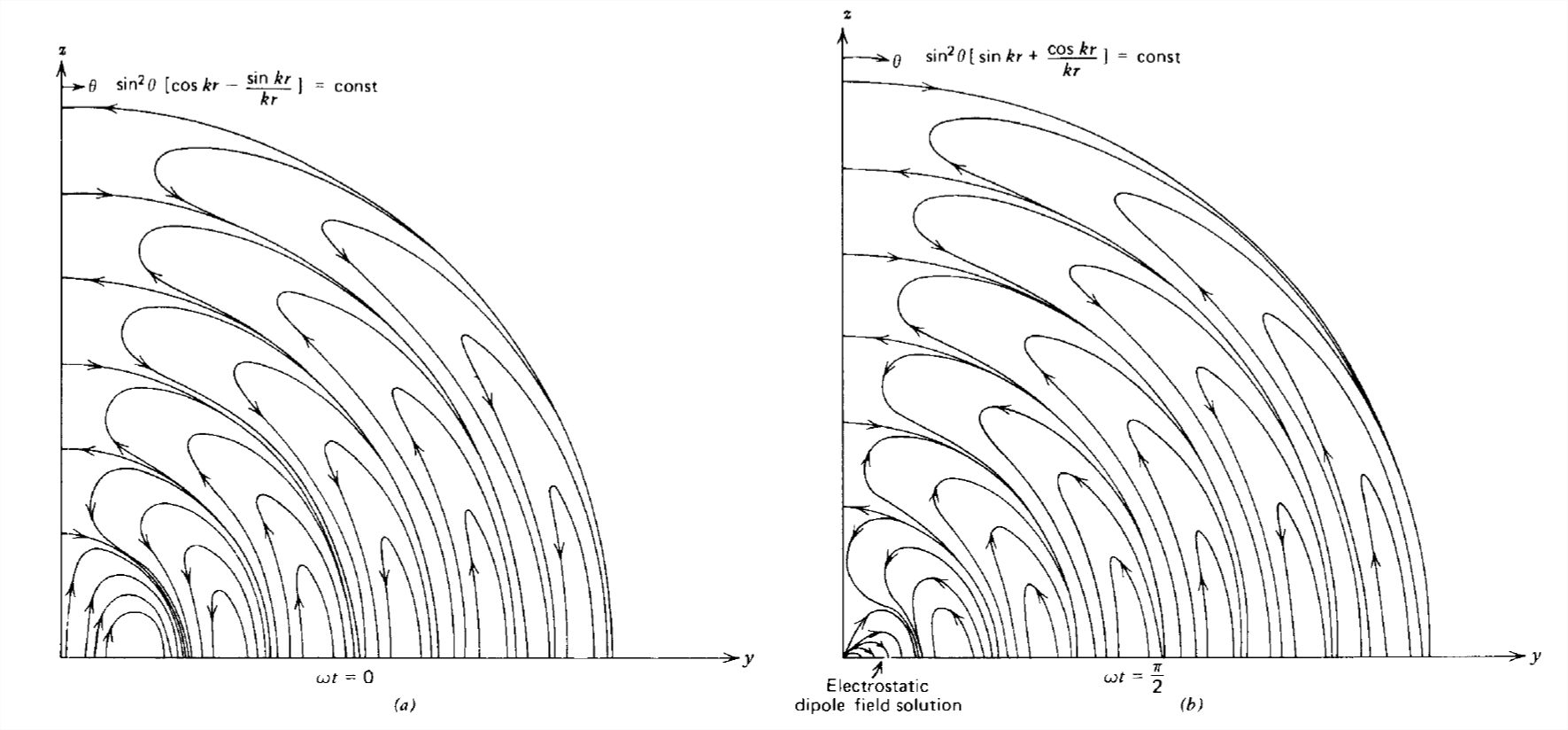
These field lines are plotted in Figure 9-2 at two values of time. We can check our result with the static field lines for a dipole given in Section 3-1-1. Remembering that \(k=\omega /c\), at low frequencies,

\[\]\[ \lim_{\omega \rightarrow 0}\left\{\begin{array}{lr}
\displaystyle \cos \left ( \omega t-kr \right )\approx 1\\ 
\displaystyle \frac{\sin \left ( \omega t-kr \right )}{kr}\approx \frac{\left ( t-r/c \right )}{r/c}\approx \frac{t}{r/c}-1
\nonumber \end{array}\right. \]

so that, in the low-frequency limit at a fixed time, (24) approaches the result of Eq. (6) of Section 3-1-1:

\[ \lim_{\omega \rightarrow 0}\sin ^{2}\theta \left ( \frac{ct}{r} \right )=\textrm{const} \]

Note that the field lines near the dipole are those of a static dipole field, as drawn in Figure 3-2. In the far field limit

\[ \lim_{kr \gg  1}\sin ^{2}\theta \cos \left ( \omega t-kr \right )=\textrm{const} \]

the field lines repeat with period \(\lambda =2\pi /k\).

Radiation Resistance

Using the electric and magnetic fields of Section 9-2-3, the time-average power density is

\[ \begin{align}<\textbf{S}>&=\frac{1}{2}\textrm{Re}\left ( \hat{\textbf{E}}\times\hat{\textbf{E}}^{\ast } \right ) \\ &
=\textrm{Re}\left \{ \frac{\left | \hat{I}dl \right |^{2}\eta k^{4}}{2\left ( 4\pi  \right )^{2}}\left [ -\textbf{i}_{\theta }\sin 2\theta \left ( -\frac{1}{\left ( jkr \right )^{3}}+\frac{1}{\left ( jkr \right )^{5}} \right ) \right ]+\textbf{i}_{r}\sin ^{2}\theta \left ( -\frac{1}{\left ( jkr \right )^{2}}+\frac{1}{\left ( jkr \right )^{5}} \right )\right \} \nonumber \\ &
=\frac{1}{2}\left | \hat{I}dl \right |^{2}\left ( \frac{k}{4\pi } \right )^{2}\frac{\eta }{r^{2}}\sin^{2}\theta \textbf{i}_{r} \nonumber \\ &
=\frac{1}{2}\frac{\left | \hat{E}_{0} \right |^{2}}{\eta }\frac{\sin ^{2}\theta }{\left ( kr \right )^{2}}\textbf{i}_{r} \nonumber \end{align} \]

where \(\hat{E}_{0}\) is defined in (16).

Only the far fields contributed to the time-average power flow. The near and intermediate fields contributed only imaginary terms in (28) representing reactive power.

The power density varies with the angle \(\theta \), being zero along the electric dipole's axis \(\left ( \theta =0,\pi  \right )\) and maximum at right angles to it \(\left ( \theta =\pi /2 \right )\), illustrated by the radiation power pattern in Fig. 9-3. The strength of the power density is proportional to the length of the vector from the origin to the

Figure 9-3 The strength of the electric field and power density due to a \(z\)-directed point dipole as a function of angle \(\theta \) is proportional to the length of the vector from the origin to the radiation pattern.

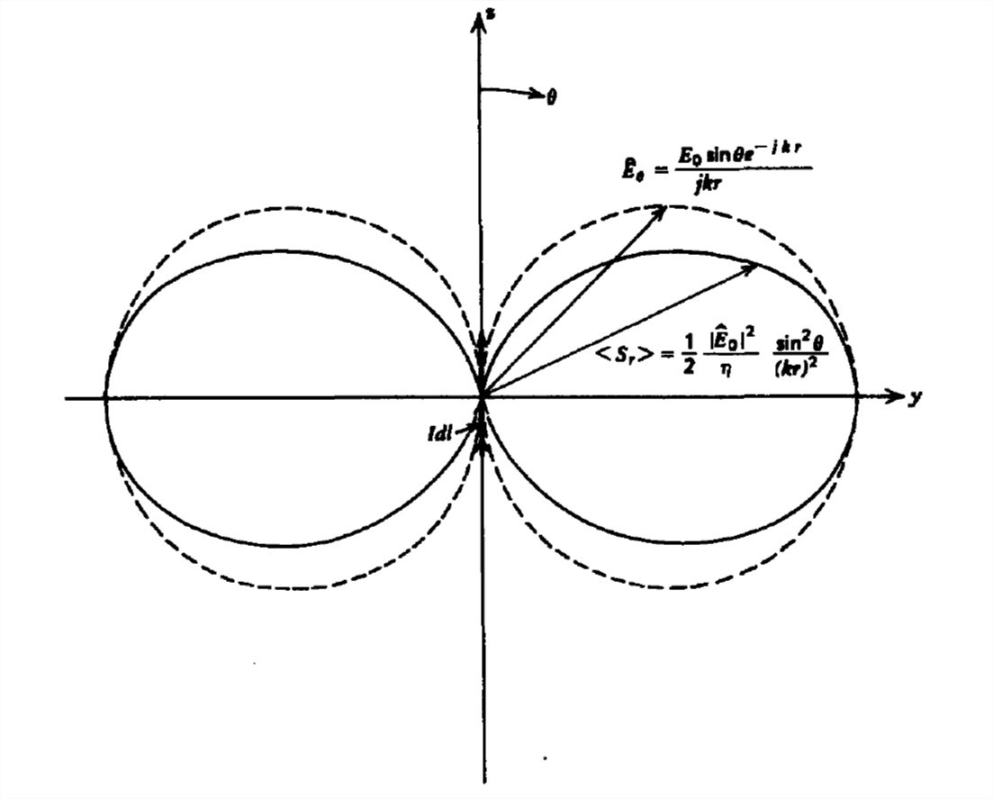
radiation pattern. These directional properties are useful in beam steering, where the directions of power Row can be controlled.

The total time-average power radiated by the electric dipole is found by integrating the Poynting vector over a spherical surface at any radius \(r\):

\[ \begin{align} <P>&=\int_{\theta =0}^{\pi }\int_{\phi =0}^{2\pi }<S_{r}>r^{2}\sin \theta d\theta d\phi \\ & =\frac{1}{2}\left | \hat{I}dl \right |^{2}\left ( \frac{k}{4\pi } \right )^{2}\eta 2\pi \int_{\theta =0}^{\pi }\sin ^{3}\theta d\theta \nonumber \\ & =\frac{\left | \hat{I}dl \right |^{2}}{16\pi }\eta k^{2}\left [ -\frac{1}{3}\cos \theta \left ( \sin ^{2}\theta +2 \right ) \right ]\bigg|_{0}^{\pi } \nonumber \\ & =\frac{\left | \hat{I}dl \right |^{2}}{12\pi }\eta k^{2} \nonumber \end{align} \]

As far as the dipole is concerned, this radiated power is lost in the same way as if it were dissipated in a resistance \(R\),

\[ <P>=\frac{1}{2}\left | \hat{I} \right |^{2}R \]

where this equivalent resistance is called the radiation resistance:

\[ R=\frac{\eta }{6\pi }\left ( k\,dl \right )^{2}=\frac{2\pi \eta }{3}\left ( \frac{dl}{\lambda } \right )^{2},\quad k=\frac{2\pi }{\lambda } \]

In free space \(\eta _{0}=\sqrt{\mu _{0}/\varepsilon _{0}}\approx 120\pi \), the radiation resistance is

\[ R_{0}=80\pi^{2}\left ( \frac{dl}{\lambda} \right )^{2}\quad \left ( \textrm{free space} \right ) \]

These results are only true for point dipoles, where \(dl\) is much less than a wavelength \(\left ( dl/\lambda \ll 1 \right )\). This verifies the validity of the quasi-static approximation for geometries much smaller than a radiated wavelength, as the radiated power is then negligible.

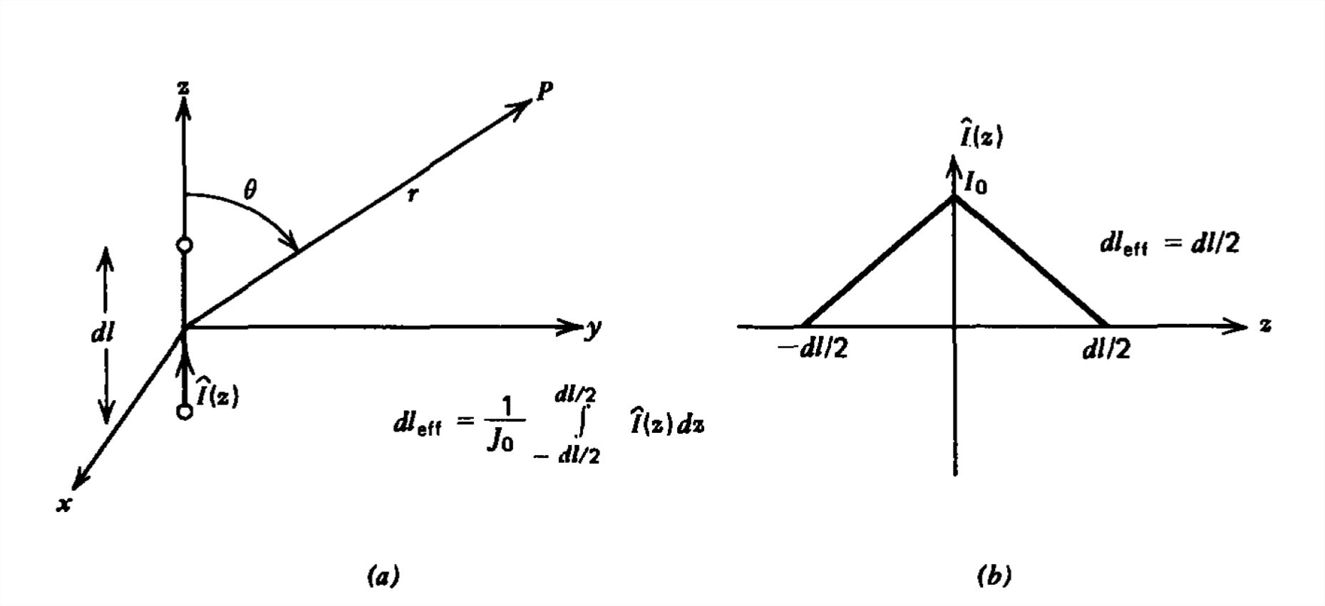
If the current on a dipole is not constant but rather varies with \(z\) over the length, the only term that varies with \(z\) for the vector potential in (5) is \(\hat{I}\left ( z \right )\):

\[ \hat{A}_{z}\left ( r \right )=\textrm{Re}\left [ \int_{-dl/2}^{+dl/2}\frac{\mu \hat{I}\left ( z \right )e^{-jkr_{\mathcal{Q}P}}}{4\pi r_{\mathcal{Q}P}}dz \right ]\approx \textrm{Re}\left [ \frac{\mu e^{-jkr_{\mathcal{Q}P}}}{4\pi r_{\mathcal{Q}P}}\int_{-dl/2}^{+dl/2}\hat{I}\left ( z \right )dz \right ]  \]

where, because the dipole is of infinitesimal length, the distance \(r_{\mathcal{Q}P}\) from any point on the dipole to any field point far from the dipole is essentially \(r\), independent of \(z\). Then, all further results for the electric and magnetic fields are the same as in Section 9-2-3 if we replace the actual dipole length \(dl\) by its effective length,

\[ dl_{\textrm{eff}}=\frac{1}{\hat{I}_{0}}\int_{-dl/2}^{+dl/2}\hat{I}\left ( z \right )dz \]

where \(\hat{I}_{0}\) is the terminal current feeding the center of the dipole.

Generally the current is zero at the open circuited ends, as for the linear distribution shown in Figure 9-4,

\[ \hat{I}\left ( z \right )=\left\{\begin{array}{ll}
\displaystyle I_{0}\left ( 1-2z/dl \right ),\quad 0\leq z\leq dl/2\\ 
\displaystyle I_{0}\left ( 1-2z/dl \right ),\quad -dl/2\leq z\leq 0
\end{array}\right.  \]

so that the effective length is half the actual length:

\[ dl_{\textrm{eff}}=\frac{1}{I_{0}}\int_{-dl/2}^{+dl/2}\hat{I}\left ( z \right )dz=\frac{dl}{2} \]

Figure 9-4 (a) If a point electric dipole has a nonuniform current distribution, the solutions are of the same form if we replace the actual dipole length \(dl\) by an effective length \(dl_{\textrm{eff}}\). (b) For a triangular current distribution the effective length is half the true length.

Because the fields are reduced by half, the radiation resistance is then reduced by :

\[ R=\frac{2\pi \eta }{3}\left ( \frac{dl_{\textrm{eff}}}{\lambda } \right )^{2}=20\pi ^{2}\sqrt{\frac{\mu _{r}}{\varepsilon _{r}}}\left ( \frac{dl}{\lambda } \right )^{2} \]

In free space the relative permeability \(\mu _{r}\) and relative permittivity \(\varepsilon _{r}\) are unity.

Note also that with a spatially dependent current distribution, a line charge distribution is found over the whole length of the dipole and not just on the ends:

\[ \hat{\lambda }=-\frac{1}{j\omega }\frac{d\hat{I}}{dz} \]

For the linear current distribution described by (35), we see that:

\[ \hat{\lambda }=\pm \frac{2I_{0}}{j\omega dl}\left\{\begin{matrix}
0\leq z\leq dl/2\\ 
-dl/2\leq z\leq 0
\end{matrix}\right. \]

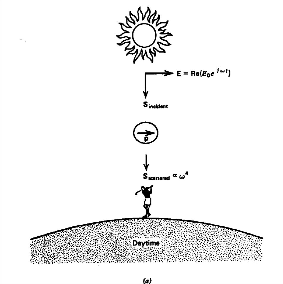
Rayleigh Scattering (or why is the sky blue?)

If a plane wave electric field \(\textrm{Re}\left [ E_{0}e^{j\omega t} \textbf{i}_{x}\right ]\) is incident upon an atom that is much smaller than the wavelength, the induced dipole moment also contributes to the resultant field, as illustrated in Figure 9-5. The scattered power is perpendicular to the induced dipole moment. Using the dipole model developed in Section 3-1-4, where a negative spherical electron cloud of radius \(R_{0}\) with total charge \(-\mathcal{Q}\) surrounds a fixed

Figure 9-5 An incident electric field polarizes dipoles that then re-radiate their energy primarily perpendicular to the polarizing electric field. The time-average scattered power increases with the fourth power of frequency so shorter wavelengths of light are scattered more than longer wavelengths. (a) During the daytime an earth observer sees more of the blue scattered light so the sky looks blue (short wavelengths). (b) Near sunset the light reaching the observer lacks blue so the sky appears reddish (long wavelength).

positive point nucleus, Newton's law for the charged cloud with mass \(m\) is:

\[ \frac{d^{2}x}{dt^{2}}+\omega _{0}^{2}x=\textrm{Re}\left ( \frac{\mathcal{Q}E_{0}}{m}e^{j\omega t} \right ),\quad \omega _{0}^{2}=\frac{\mathcal{Q}^{2}}{4\pi \varepsilon mR_{0}^{3}} \]

The resulting dipole moment is then

\[  \hat{p}=\mathcal{Q}\hat{x}=\frac{\mathcal{Q}^{2}E_{0}/m}{\omega_{0}^{2}-\omega^{2}} \]

where we neglect damping effects. This dipole then re-radiates with solutions given in Sections 9-2-1-9-2-5 using the dipole moment of (41) \(\left ( \hat{I}dl\rightarrow j\omega\hat{p} \right )\). The total time-average power radiated is then found from (29) as

\[ <P>=\frac{\omega ^{4}\left | \hat{p} \right |^{2}\eta }{12\pi c^{2}}=\frac{\omega ^{4}\eta \left ( \mathcal{Q}^{2}E_{0}/m\right )^{2}}{12\pi c^{2}\left ( \omega _{0}^{2}-\omega ^{2} \right )^{2}} \]

To approximately compute \(\omega _{0}\), we use the approximate radius of the electron found in Section 3-8-2 by equating the energy stored in Einstein's relativistic formula relating mass to energy:

\[ mc^{2}=\frac{3Q^{2}}{20\pi \varepsilon R_{0}}\Rightarrow R_{0}=\frac{3Q^{2}}{20\pi \varepsilon mc^{2}}\approx 1.69\times 10^{-15}m  \]

Then from (40)

\[ \omega _{0}=\frac{\sqrt{5/3}20\pi \varepsilon mc^{2}}{3\mathcal{Q}^{2}}\approx 2.3\times 10^{23}\,\textrm{radian/sec} \]

is much greater than light frequencies \(\left ( \omega \approx 10^{15} \right )\) so that (42) becomes approximately

\[ \lim_{\omega _{0}\gg \omega }<P>\approx \frac{\eta }{12\pi }\left ( \frac{\mathcal{Q}^{2}E_{0}\omega ^{2}}{mc\omega _{0}^{2}} \right )^{2} \]

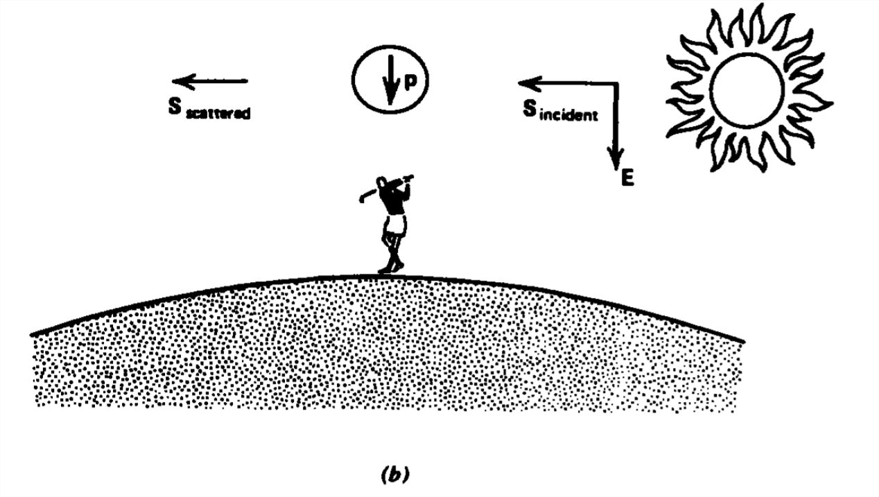
This result was originally derived by Rayleigh to explain the blueness of the sky. Since the scattered power is proportional to \(\omega ^{4}\), shorter wavelength light dominates. However, near sunset the light is scattered parallel to the earth rather than towards it. The blue light received by an observer at the earth is diminished so that the longer wavelengths dominate and the sky appears reddish.

Radiation from a Point Magnetic Dipole

A closed sinusoidally varying current loop of very small size flowing in the \(z = 0\) plane also generates radiating waves. Because the loop is closed, the current has no divergence so that there is no charge and the scalar potential is zero. The vector potential phasor amplitude is then

\[ \hat{\textbf{A}}\left ( r \right )=\int \frac{\mu \hat{\textbf{I}}e^{-jkr_{\mathcal{Q}P}}}{4\pi r_{\mathcal{Q}P}}dl \]

We assume the dipole to be much smaller than a wavelength, \(k\left ( r_{\mathcal{Q}P}-r\right )\ll 1\), so that the exponential factor in (46) can be linearized to

\[ \lim_{k\left ( r_{\mathcal{Q}P}-r \right )\ll 1}e^{-jkr_{\mathcal{Q}P}}=e^{-jkr}e^{-jk\left ( r_{\mathcal{Q}P}-r \right )}\approx e^{-jkr}\left [ 1-jk\left ( r_{\mathcal{Q}P}-r \right ) \right ] \]

Then (46) reduces to

\[ \begin{align} \hat{\textbf{A}}\left ( r \right )&=\int \frac{\mu \hat{\textbf{I}}}{4\pi }e^{-jkr}\left ( \frac{1+jkr}{r_{\mathcal{Q}P}} -jk\right )dl \\ & =e^{-jkr}\int \frac{\mu \hat{\textbf{I}}}{4\pi }\left ( \frac{1+jkr}{r_{\mathcal{Q}P}} -jk\right )dl \nonumber \\ &=\frac{\mu}{4\pi }e^{-jkr}\left ( \left ( 1+jkr \right )\int \frac{\hat{\textbf{I}}dl}{r_{\mathcal{Q}P}}-jk\int \hat{\textbf{I}}dl \right ) \nonumber \end{align} \]

where all terms that depend on \(r\) can be taken outside the integrals because \(r\) is independent of \(dl\). The second integral is zero because the vector current has constant magnitude and flows in a closed loop so that its average direction integrated over the loop is zero. This is most easily seen with a rectangular loop where opposite sides of the loop contribute equal magnitude but opposite signs to the integral, which thus sums to zero. If the loop is circular with radius \(a\),

\[ \hat{\textbf{I}}dl=\hat{I}\textbf{i}_{\phi }ad\phi \Rightarrow \int_{0}^{2\pi }\textbf{i}_{\phi }d\phi =\int_{0}^{2\pi }\left ( -\sin \phi \textbf{i}_{x}+\cos \phi \textbf{i}_{y} \right )d\phi =0 \]

the integral is again zero as the average value of the unit vector \(\textbf{i}_{\phi }\) around the loop is zero.

The remaining integral is the same as for quasi-statics except that it is multiplied by the factor \(\left ( 1+jkr \right )e^{-jkr}\). Using the results of Section 5-5-1, the quasi-static vector potential is also multiplied by this quantity:

\[ \hat{\textbf{A}}=\frac{\mu \hat{m}}{4\pi r^{2}}\sin \theta \left ( 1+jkr \right )e^{-jkr}\textbf{i}_{\phi },\quad \hat{m}=\hat{I}dS \]

The electric and magnetic fields are then

\[ \hat{\textbf{H}}=\frac{1}{\mu }\nabla \times \hat{\textbf{A}}=-\frac{\hat{m}}{4\pi }jk^{3}e^{-jkr}\left \{ \textbf{i}_{r}\left [ 2\cos \theta \left ( \frac{1}{\left ( jkr \right )^{2}}+\frac{1}{\left ( jkr \right )^{3}} \right ) \right ]+\textbf{i}_{\theta }\left [ \sin \theta \left ( \frac{1}{ jkr}+\frac{1}{\left ( jkr \right )^{2}}+\frac{1}{\left ( jkr \right )^{3}} \right ) \right ] \right \}\\
\hat{\textbf{E}}=\frac{1}{j\omega \varepsilon }\nabla \times \hat{\textbf{H}}=\frac{\hat{m}jk^{3}}{4\pi }\eta e^{-jkr}\sin \theta \left ( \frac{1}{ jkr}+\frac{1}{\left ( jkr \right )^{2}} \right )\textbf{i}_{\phi } \]

The magnetic dipole field solutions are the dual to those of the electric dipole where the electric and magnetic fields reverse roles if we replace the electric dipole moment with the magnetic dipole moment:

\[ \frac{\textbf{p}}{\varepsilon }=\frac{q\textbf{dl}}{\varepsilon }=\frac{\textbf{I}dl}{j\omega \varepsilon }\rightarrow \textbf{m} \]