9.3: Point Dipole Arrays

The power density for a point electric dipole varies with the broad angular distribution \(\sin ^{2}\theta \). Often it is desired that the power pattern be highly directive with certain angles carrying most of the power with negligible power density at other angles. It is also necessary that the directions for maximum power flow be controllable with no mechanical motion of the antenna. These requirements can be met by using more dipoles in a periodic array.

A Simple Two Element Array

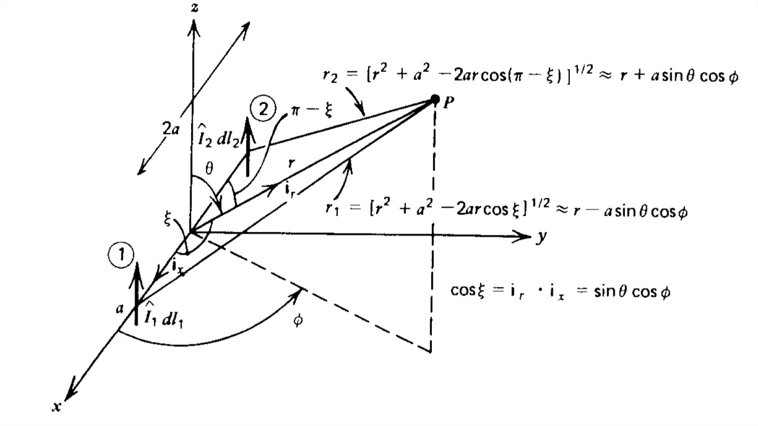
To illustrate the basic principles of antenna arrays we consider the two element electric dipole array shown in Figure 9-6. We assume each element carries uniform currents \(\hat{I}_{1}\) and \(\hat{I}_{2}\) and has lengths \(dl_{1}\) and \(dl_{2}\), respectively. The elements are a distance \(2a\) apart. The fields at any point \(P\) are given by the superposition of fields due to each dipole alone. Since we are only interested in the far field radiation pattern where \(\theta _{1}\approx \theta _{2}\approx \theta \), we use the solutions of Eq. (16) in Section 9-2-3 to write:

\[\hat{E}_{\theta }=\eta \hat{H}_{\phi }=\frac{\hat{E}_{1}\sin \theta e^{-jkr_{1}}}{jkr_{1}}+\frac{\hat{E}_{2}\sin \theta e^{-jkr_{2}}}{jkr_{2}} \]

where

\(\hat{E}_{1}=-\frac{\hat{I}_{1}dl_{1}k^{2}}{4\pi }\eta ,\quad \hat{E}_{2}=-\frac{\hat{I}_{2}dl_{2}k^{2}\eta }{4\pi }\)

Figure 9-6 The field at any point \(P\) due to two-point dipoles is just the sum of the fields due to each dipole alone taking into account the difference in distances to each dipole.

Remember, we can superpose the fields but we cannot superpose the power flows.

From the Law of Cosines the distances \(r_{1}\), and \(r_{2}\) are related as

\[ \begin{align}r_{2}&=\left [ r^{2}+a^{2}-2ar\cos \left ( \pi -\xi  \right ) \right ]^{1/2}=\left [ r^{2}+a^{2}+2ar\cos \xi  \right ]^{1/2} \\
r_{1}&=\left [ r^{2}+a^{2}-2ar\cos \xi  \right ]^{1/2} \nonumber \end{align} \]

where \(\xi\) is the angle between the unit radial vector \(\textbf{i}_{r}\) and the \(x\) axis:

\( \cos \xi =\textbf{i}_{r}\cdot \textbf{i}_{x}=\sin \theta \cos \phi \)

Since we are interested in the far field pattern, we linearize (2) to

\[\lim_{r\gg a}\left\{\begin{matrix}
\displaystyle r_{2}\approx r\left [ 1+\frac{1}{2}\left ( \frac{a^{2}}{r^{2}}+\frac{2a}{r}\sin \theta \cos \phi  \right ) \right ]\approx r+a\sin \theta \cos \phi \\ 
\displaystyle r_{1}\approx r\left [ 1+\frac{1}{2}\left ( \frac{a^{2}}{r^{2}}-\frac{2a}{r}\sin \theta \cos \phi  \right ) \right ]\approx r-a\sin \theta \cos \phi 
\end{matrix}\right.   \]

In this far field limit, the correction terms have little effect in the denominators of (1) but can have significant effect in the exponential phase factors if \(a\) is comparable to a wavelength so that \(ka\) is near or greater than unity. In this spirit we include the first-order correction terms of (3) in the phase factors of (1), but not anywhere else, so that (1) is rewritten as

\[ \begin{align} \hat{E}_{\theta }&=\eta \hat{H}_{\phi } \\ &
=\underset{\textrm{element facotr}}{\underbrace{\frac{jk\eta }{4\pi r}\sin \theta e^{-jkr}}}\underset{\textrm{array factor}}{\underbrace{\left ( \hat{I}_{1}dl_{1}e^{jka\sin \theta \cos \phi }+\hat{I}_{2}dl_{2}e^{-jka\sin \theta \cos \phi } \right )}} \nonumber \end{align} \]

The first factor is called the element factor because it is the radiation field per unit current element \(\left ( \hat{I}dl \right )\) due to a single dipole at the origin. The second factor is called the array factor because it only depends on the geometry and excitations (magnitude and phase) of each dipole element in the array.

To examine (4) in greater detail, we assume the two dipoles are identical in length and that the currents have the same magnitude but can differ in phase \(\mathcal{X}\):

\[ dl_{1}=dl_{2}\equiv dl\\
\hat{I}_{1}=\hat{I},\quad \hat{I}_{2}=\hat{I}e^{j\mathcal{X}}\Rightarrow \hat{E}_{1}=\hat{E}_{0},\quad \hat{E}_{2}=\hat{E}_{0}e^{j\mathcal{X}} \]

so that (4) can be written as

\[ \hat{E}_{\theta }=\eta \hat{H}_{\phi }=\frac{2\hat{E}_{0}}{jkr}e^{-jkr}\sin \theta e^{j\mathcal{X}/2}\cos \left ( ka\sin \theta \cos \phi -\frac{\mathcal{X}}{2} \right ) \]

Now the far fields also depend on \(\phi \). In particular, we focus attention on the \(\theta =\pi /2\) plane. Then the power flow,

\[ \lim_{\theta =\pi /2}<S_{r}>=\frac{1}{2\eta }\left | \hat{E}_{\theta} \right |^{2}=\frac{2\left | \hat{E}_{0} \right |^{2}}{\eta \left ( kr \right )^{2}}\cos ^{2}\left ( ka\cos \phi -\frac{\mathcal{X}}{2} \right ) \]

depends strongly on the dipole spacing \(2a\) and current phase difference \(\mathcal{X}\).

(a) Broadside Array

Consider the case where the currents are in phase \(\left ( \mathcal{X}=0 \right )\) but the dipole spacing is a half wavelength \(\left ( 2a=\lambda /2 \right )\). Then, as illustrated by the radiation pattern in Figure 9-7a, the field strengths cancel along the \(x\) axis while they add along the \(y\) axis. This is because along the \(y\) axis \(r_{1}=r_{2}\), so the fields due to each dipole add, while along the \(x\) axis the distances differ by a half wavelength so that the dipole fields cancel. Wherever the array factor phase \(\left ( ka\cos \phi -\mathcal{X}/2 \right )\) is an integer multiple of \(\pi \), the power density is maximum, while wherever it is an odd integer multiple of \(\pi /2\), the power density is zero. Because this radiation pattern is maximum in the direction perpendicular to the array, it is called a broadside pattern.

Figure 9-7 The power radiation pattern due to two-point dipoles depends strongly on the dipole spacing and current phases. With a half wavelength dipole spacing \(\left ( 2a=\lambda /2 \right )\), the radiation pattern is drawn for various values of current phase difference in the \(\theta =\pi /2\) plane. The broadside array in (a) with the currents in phase \(\left ( \mathcal{X}=0 \right )\) has the power lobe in the direction perpendicular to the array while the end-fire array in (e) has out-of-phase currents \(\left ( \mathcal{X}= \pi \right )\) with the power lobe in the direction along the array.

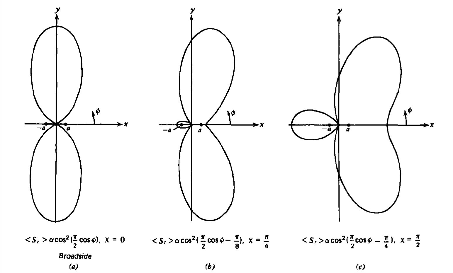
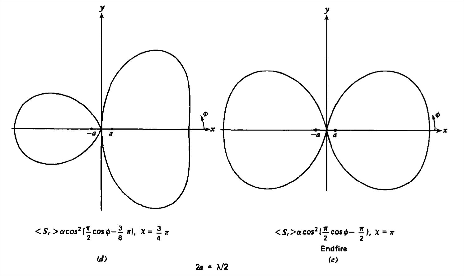
(b) End-fire Array

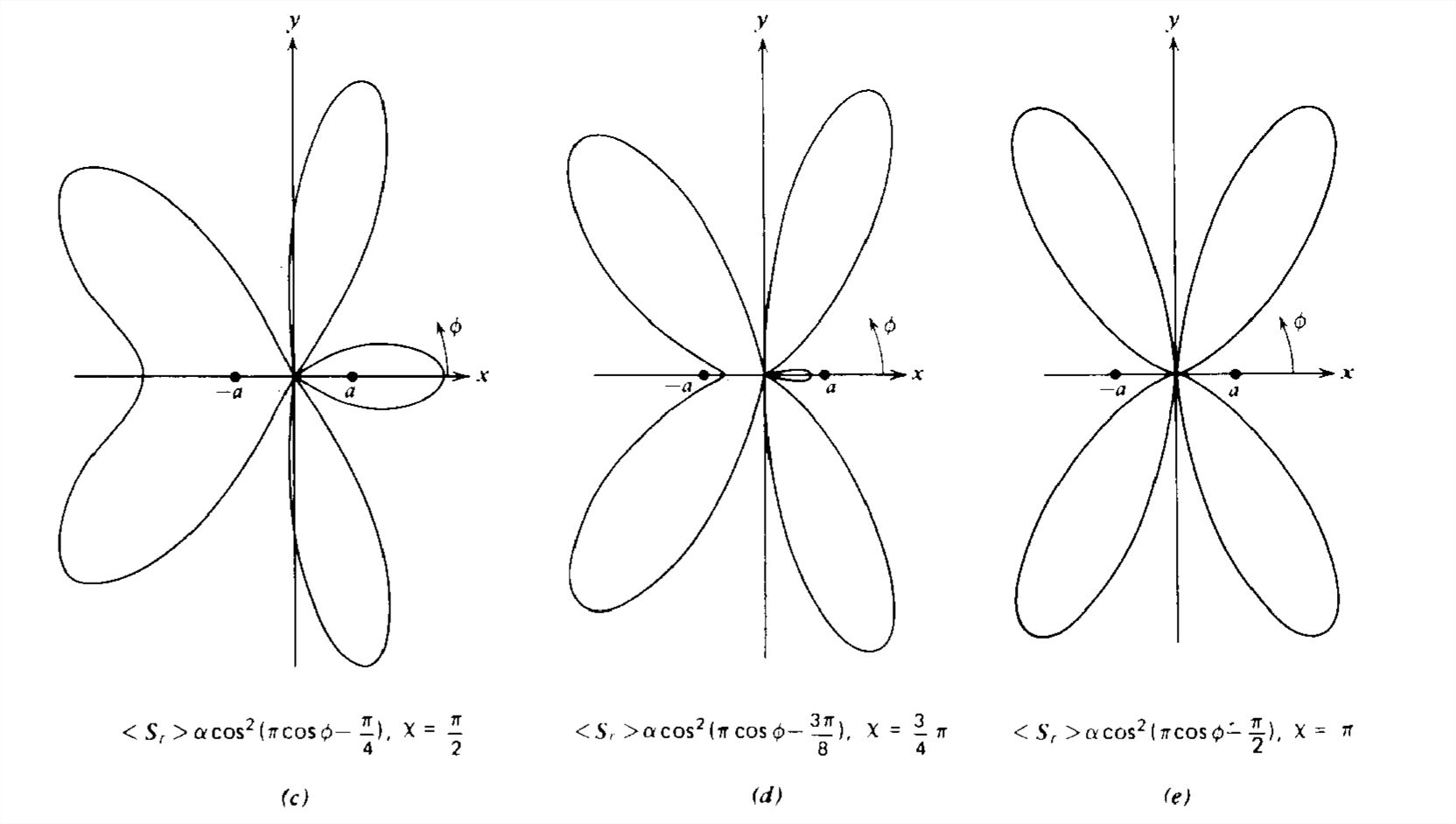
If, however, for the same half wavelength spacing the currents are out of phase \(\left ( \mathcal{X}= \pi \right )\), the fields add along the \(x\) axis but cancel along the \(y\) axis. Here, even though the path lengths along the \(y\) axis are the same for each dipole, because the currents are out of phase the fields cancel. Along the \(x\) axis the extra \(\pi\) phase because of the half wavelength path difference is just canceled by the current phase difference of \(\pi\) so that the fields due to each dipole add. The radiation pattern is called end-fire because the power is maximum in the direction along the array, as shown in Figure 9-7e.

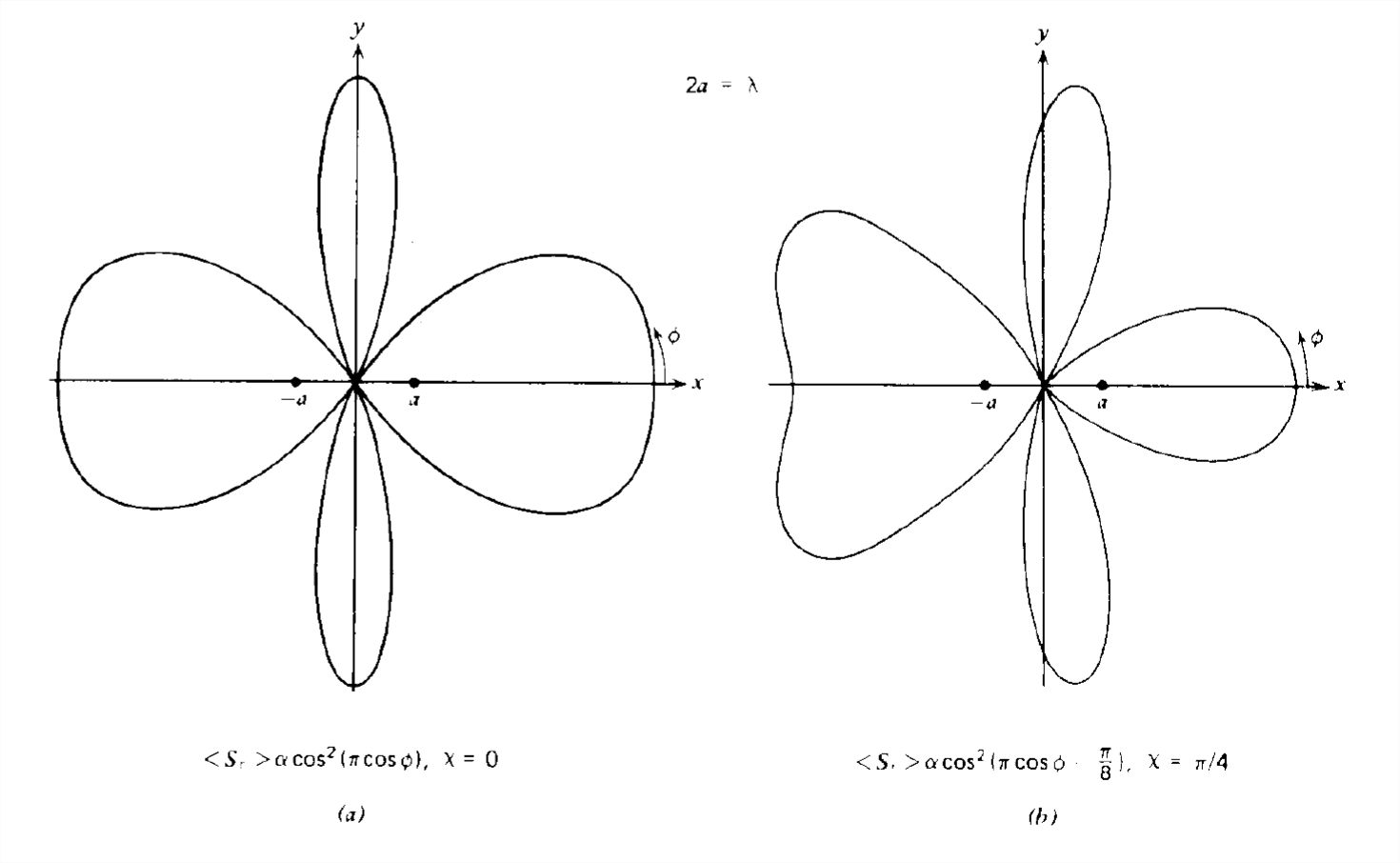
(c) Arbitrary Current Phase

For arbitrary current phase angles and dipole spacings, a great variety of radiation patterns can be obtained, as illustrated by the sequences in Figures 9-7 and 9-8. More power lobes appear as the dipole spacing is increased.

An N Dipole Array

If we have \((2N+ 1)\) equally spaced dipoles, as shown in Figure 9-9, the \(n\)th dipole's distance to the far field point is approximately,

\[ \lim_{r\gg \left | na \right |}r_{n}\approx r-na\sin \theta \cos \phi  \]

so that the array factor of (4) generalizes to

\[ AF=\sum_{-N}^{+N}\hat{I}_{n}dl_{n}e^{jkna\sin \theta \cos \phi } \]

where for symmetry we assume that there are as many dipoles to the left (negative \(n\)) as to the right (positive \(n\)) of the \(z\) axis, including one at the origin \((n = 0)\). In the event that a dipole is not present at a given location, we simply let its current be zero. The array factor can be varied by changing the current magnitude or phase in the dipoles. For simplicity here, we assume that all dipoles have the same length \(dl\), the same current magnitude \(\hat{I}_{0}\), and differ in phase from its neighbors by a constant angle \(\mathcal{X}_{0}\) so that

\[ \hat{I}_{n}=I_{0}e^{-jn\mathcal{X}_{0}},\quad -N\leq N \]

and (9) becomes

\[ AF=I_{0}dl\sum_{-N}^{+N}e^{jn}\left ( ka\sin \theta \cos \phi -\mathcal{X}_{0} \right ) \]

Figure 9-8 With a full wavelength dipole spacing \(\left ( 2a=\lambda  \right )\) there are four main power lobes.

Defining the parameter

\[ \beta =e^{j\left ( ka\sin \theta \cos \phi -\mathcal{X}_{0} \right )} \]

the geometric series in (11) can be written as

\[ S=\sum_{-N}^{+N}\beta ^{n}=\beta ^{-N}+\beta ^{-N+1}+\cdots +\beta ^{-2}+\beta ^{-1}+1+\beta +\beta ^{2}+\cdots +\beta ^{N-1}+\beta ^{N} \]

If we multiply this series by \(\beta\) and subtract from (13), we have

\[S\left ( 1-\beta  \right )=\beta ^{-N}-\beta ^{N+1} \]

which allows us to write the series sum in closed form as

\[ S=\frac{\beta ^{-N}-\beta ^{N+1}}{1-\beta }=\frac{\beta ^{-\left (N+1/2  \right )}-\beta ^{\left (N+1/2  \right )}}{\beta ^{-1/2}-\beta ^{-1/2}} =\frac{\sin \left [ \left ( N+\frac{1}{2}\right )\left ( ka\sin \theta \cos \phi -\mathcal{X}_{0} \right ) \right ]}{\sin \left [\frac{1}{2}\left ( ka\sin \theta \cos \phi -\mathcal{X}_{0} \right ) \right ]} \]

In particular, we again focus on the solution in the \(\theta =\pi /2\) plane so that the array factor is

\[ AF=I_{0}dl\frac{\sin \left [ \left ( N+\frac{1}{2} \right )\left ( ka\cos \phi -\mathcal{X}_{0} \right ) \right ]}{\sin \left [ \frac{1}{2}\left ( ka\cos \phi -\mathcal{X}_{0} \right ) \right ]} \]

The radiation pattern is proportional to the square of the array factor. Maxima occur where

\[ ka\cos \phi -\mathcal{X}_{0} =2n\pi \quad n=0,1,2... \]

The principal maximum is for \(n =0\) as illustrated in Figure 9-10 for various values of \(ka\) and \(\mathcal{X}_{0}\). The larger the number of dipoles \(N\), the narrower the principal maximum with smaller amplitude side lobes. This allows for a highly directive beam at angle \(\phi \) controlled by the incremental current phase angle \(\mathcal{X}_{0}\), so that \(\cos \phi =\mathcal{X}_{0}/ka\), which allows for electronic beam steering by simply changing \(\mathcal{X}_{0}\).