9.4: Long Dipole Antennas

The radiated power, proportional to \(\left ( dl/\lambda  \right )^{2}\), is small for point dipole antennas where the dipole's length \(dl\) is. much less than the wavelength \(\lambda \). More power can be radiated if the length of the antenna is increased. Then however, the fields due to each section of the antenna may not add constructively.

Figure 9-9 A linear point dipole array with \(2N+1\) equally spaced dipoles

Far Field Solution 

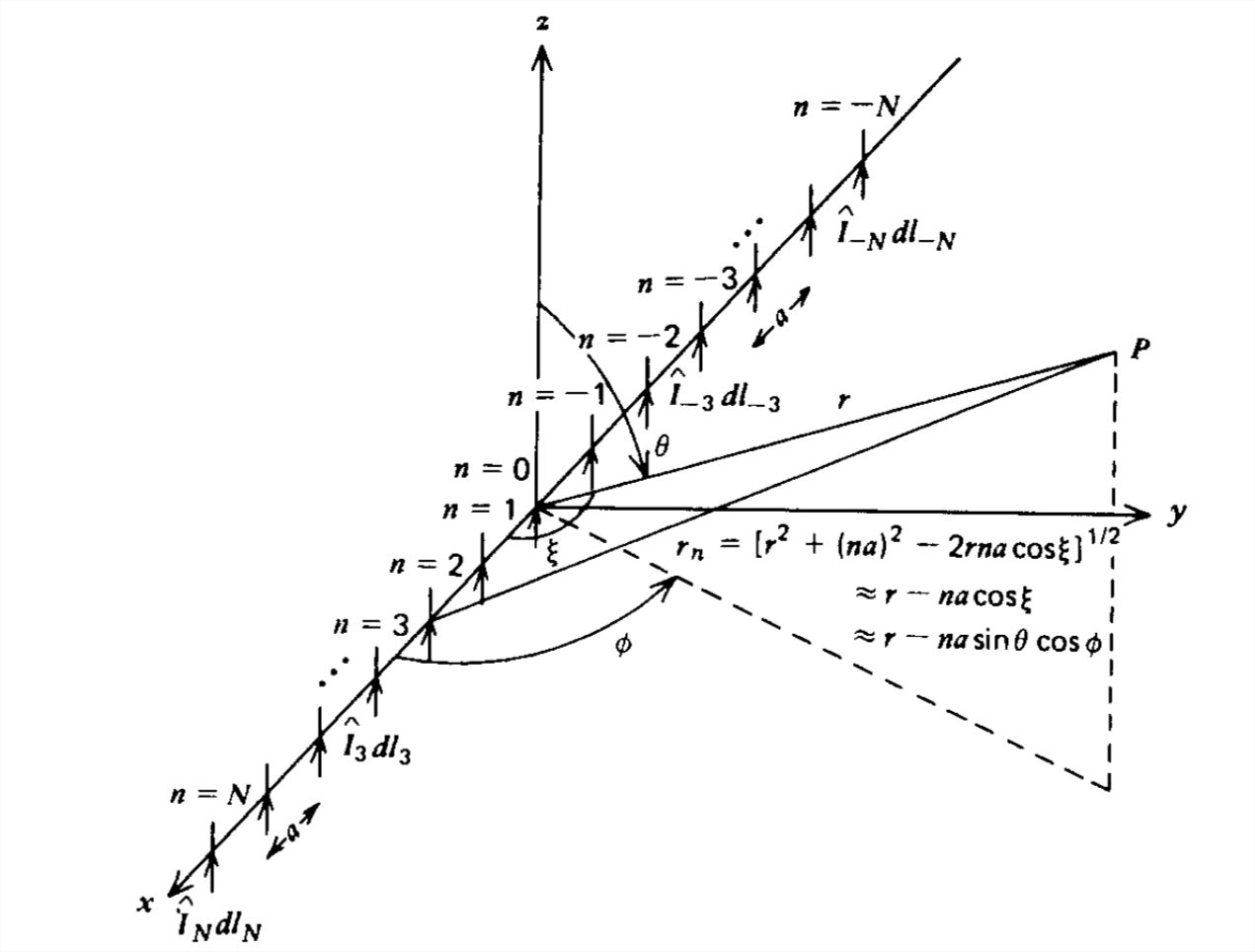
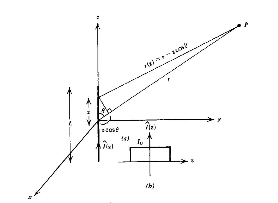
Consider the long dipole antenna in Figure 9-11 carrying a current \(\hat{I}_{z}\). For simplicity we restrict ourselves to the far field pattern where \(r\gg L\). Then, as we found for dipole arrays, the differences in radial distance for each incremental current element of length \(dz\) are only important in the exponential phase factors and not in the \(1/r\) dependences.

From Section 9-2-3, the incremental current element at position \(z\) generates a far electric field:

\[ d\hat{E}_{\theta }=\eta d\hat{H}_{\phi }=\frac{jk\eta }{4\pi }\frac{\hat{I}\left ( z \right )dz}{r}\sin \theta e^{-jk\left ( r-z\cos \theta  \right )} \]

where we again assume that in the far field the angle \(\)6 is the same for all incremental current elements.

The total far electric field due to the entire current distribution is obtained by integration over all current elements:

\[ \hat{E}_{\theta }=\eta \hat{H}_{\phi }=\frac{jk\eta }{4\pi r}\sin \theta e^{-jkr}\int_{-L/2}^{+L/2}\hat{I}\left ( z \right )e^{jkz\cos \theta }dz \]

If the current distribution is known, the integral in (2) can be directly evaluated. The practical problem is difficult because the current distribution along the antenna is determined by the near fields through the boundary conditions.

Figure 9-10 The radiation pattern for an \(N\) dipole linear array for various values of \(N\), dipole spacing \(2a\), and relative current phase \(\mathcal{X}_0\) in the \(\theta =\pi /2\) plane.

Since the fields and currents are coupled, an exact solution is impossible no matter how simple the antenna geometry. In practice, one guesses a current distribution and calculates the resultant (near and far) fields. If all boundary conditions along the antenna are satisfied, then the solution has been found. Unfortunately, this never happens with the first guess. Thus based on the field solution obtained from the originally guessed current, a corrected current distribution is used and

Figure 9-10

the resulting fields are again calculated. This procedure is numerically iterated until convergence is obtained with self-consistent fields and currents.

Uniform Current

A particularly simple case is when \(\hat{I}_{z}=\hat{I}_{0}\) is a constant.

Then (2) becomes:

\[ \begin{align}\hat{E}_{\theta }=\eta \hat{H}_{\phi }&=\frac{jk\eta }{4\pi r}\sin \theta e^{-jkr}\hat{I}_{0}\int_{-L/2}^{+L/2}e^{jkz\cos \theta} dz \\ & 
=\frac{jk\eta }{4\pi r}\sin \theta e^{-jkr}\hat{I}_{0}\frac{e^{jkz\cos \theta }}{jk\cos }\bigg|_{-L/2}^{+L/2} \nonumber \\ &
=\frac{\hat{I}_{0}\eta }{4\pi r}\tan \theta e^{-jkr}\left [ 2j\sin \left ( \frac{kL}{2}\cos \theta  \right ) \right ] \nonumber \end{align}  \]

The time-average power density is then

\[ <S_{r}>=\frac{1}{2\eta }\left | \hat{E}_{\theta } \right |^{2}=\frac{\left | \hat{E}_{0} \right |^{2}\tan ^{2}\theta \sin ^{2}\left [ \left ( kL/2 \right )\cos \theta  \right ]}{2\eta \left ( kr \right )^{2}\left ( kL/2 \right )^{2}} \]

where

\[ \hat{E}_{0}= \frac{\hat{I}_{0}L\eta k^{2}}{4\pi } \]

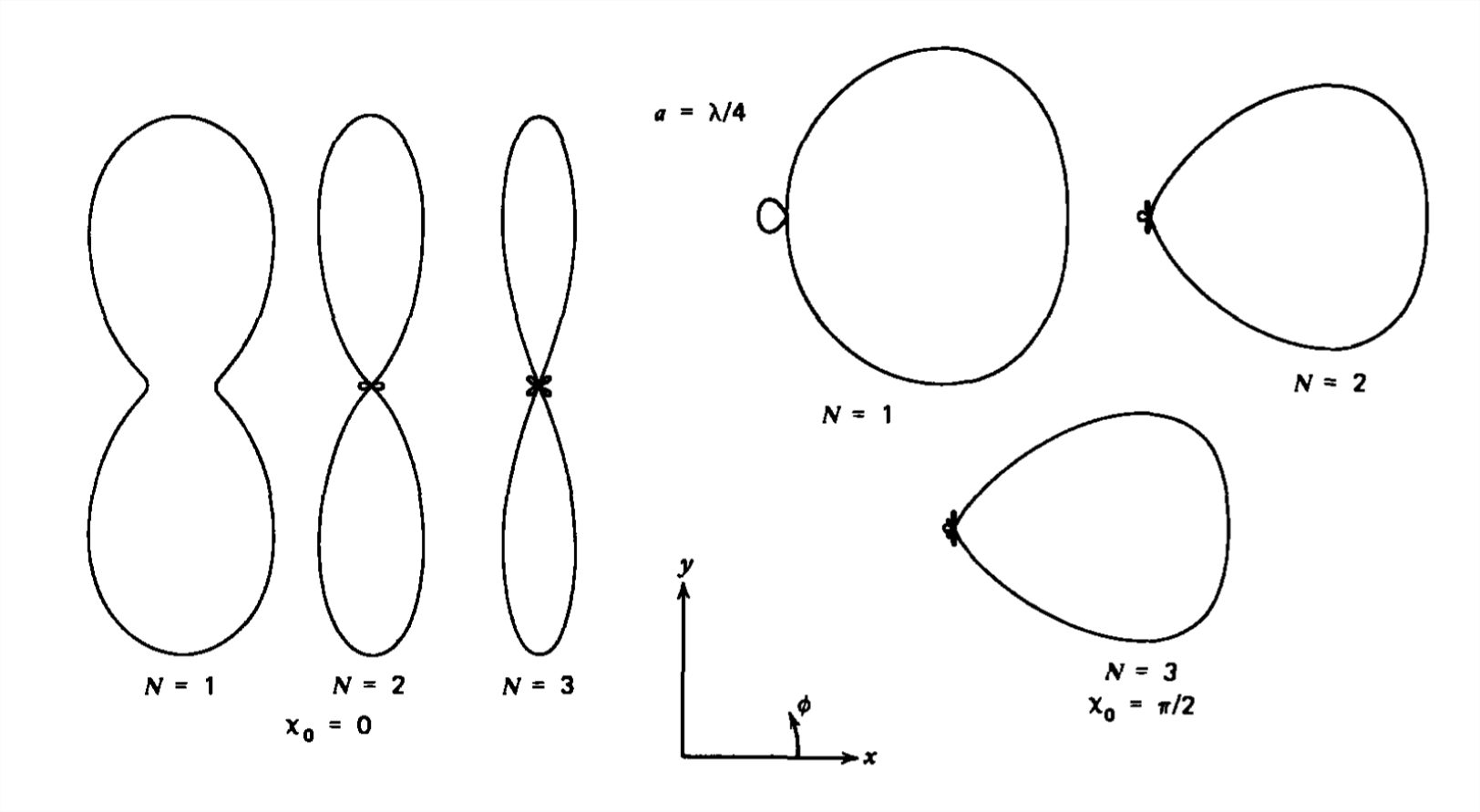
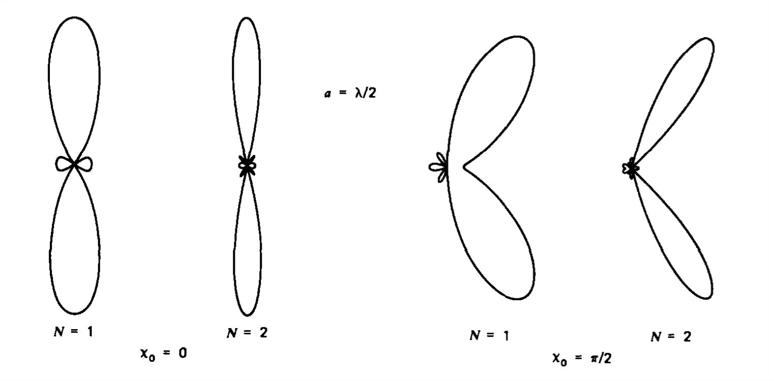
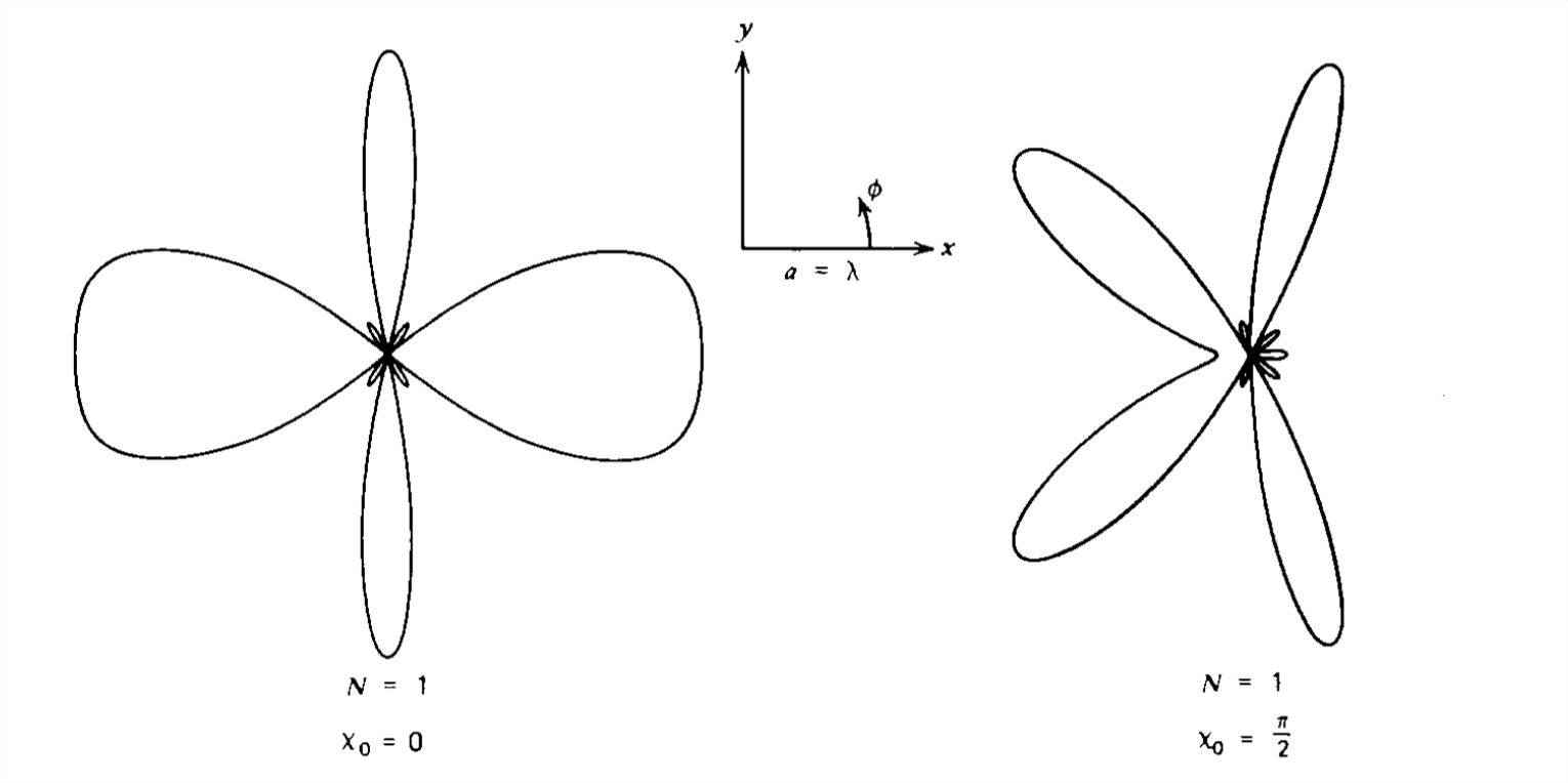
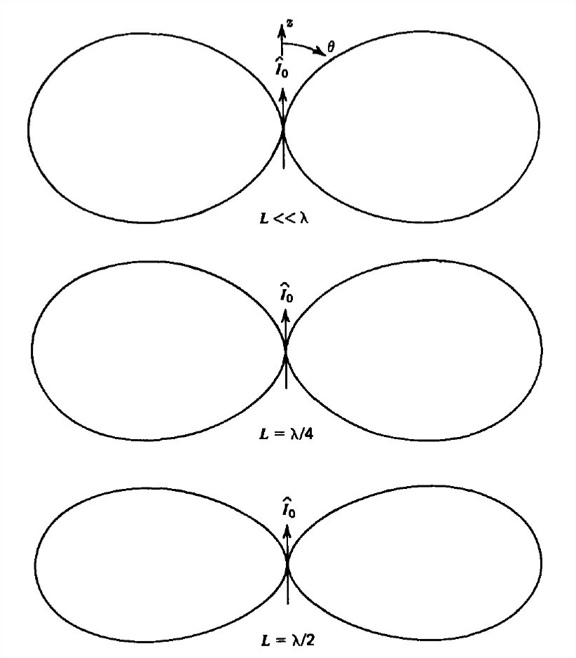
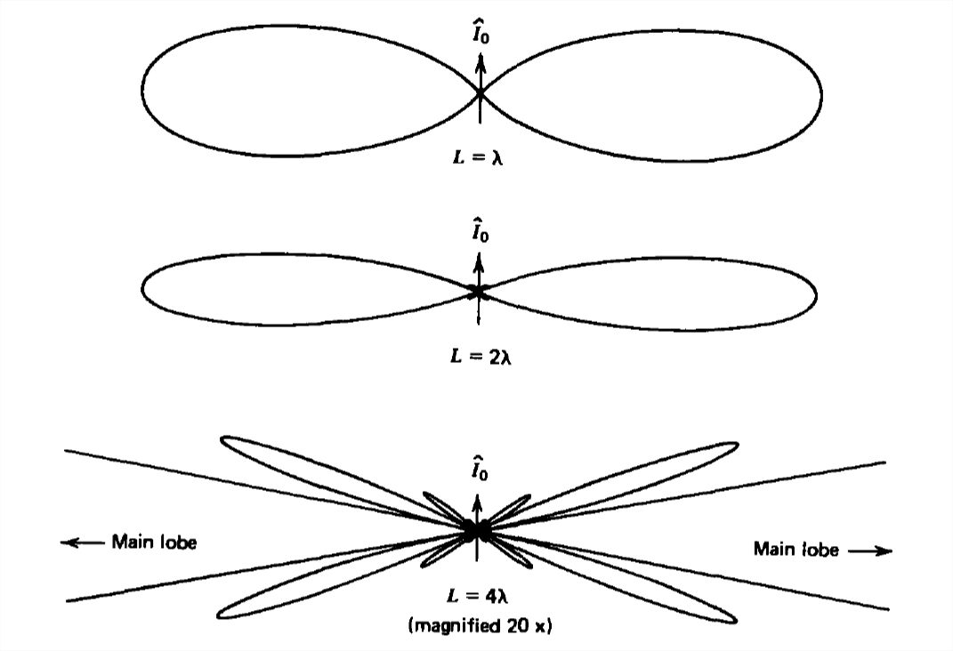
This power density is plotted versus angle \(\theta \) in Figure 9-12 for various lengths \(L\). The principal maximum always appears at \(\theta =\pi /2\), becoming sharper as \(L\) increases. For \(L >\lambda \), zero power density occurs at angles

\[ \cos \theta =\frac{2n\pi }{kL}=\frac{n\lambda }{L},\quad n=1,2,... \]

Secondary maxima then occur at nearby angles but at much smaller amplitudes compared to the main lobe at \(\theta =\pi /2\).

Radiation Resistance

The total time-average radiated power is obtained by integrating (4) over all angles:

\[ \begin{align} <P>&=\int_{\phi=0}^{2\pi }\int_{\theta =0}^{\pi }<S_{r}>r^{2}\sin \theta \,d\theta\, d\phi \\ &=\frac{\left | \hat{E}_{0} \right |^{2}\pi }{k^{2}\eta \left ( kL/2 \right )^{2}}\int_{\theta =0}^{\pi }\frac{\sin ^{3}\theta }{\cos ^{2}\theta }\sin ^{2}\left ( \frac{kL}{2}\cos \theta \right )d\theta \nonumber \end{align} \]

If we introduce the change of variable,

\[ v=\frac{kL}{2}\cos \theta ,\quad dv=-\frac{kL}{2}\sin \theta \,d\theta  \]

the integral of (7) becomes

\[ <P>=\frac{\left | \hat{E}_{0} \right |^{2}\pi }{k^{2}\eta \left ( kL/2 \right )^{2}}\int_{+kL/2}^{-kL/2}\left ( \frac{2}{kL}\sin ^{2}v\,dv-\frac{kL}{2}\frac{\sin ^{2}v}{v^{2}} \right )dv  \]

The first term is easily integrable as

\[ \int \sin ^{2}v\,dv=\frac{1}{2}v-\frac{1}{4}\sin 2v \]

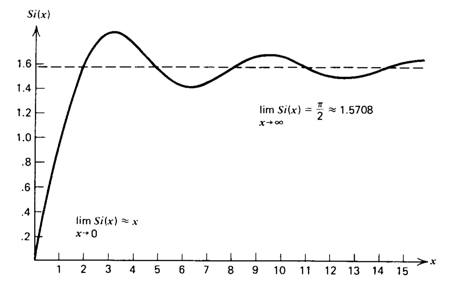
The second integral results in a new tabulated function \(\)Si(x) called the sine integral, defined as:

\[ Si\left ( x \right )=\int_{0}^{x}\frac{\sin t}{t}dt \]

Figure 9-11 (a) For a long dipole antenna, each incremental current element at coordinate \(z\) is at a slightly different distance to any field point \(P\). (b) The simplest case study has the current uniformly distributed over the length of the dipole.

which is plotted in Figure 9-13. Then the second integral in (9) can be expanded and integrated by parts:

\[ \begin{align} \int \frac{\sin ^{2}v}{v^{2}}dv&=\int \frac{\left ( 1-\cos 2v \right )}{2v^{2}}dv \\ &
=-\frac{1}{2v}-\int \cos 2v\frac{dv}{2v^{2}} \nonumber \\ &
=-\frac{1}{2v}+\frac{\cos 2v}{2v}+\int \frac{\sin 2vd\left ( 2v \right )}{2v} \nonumber \\ &
=-\frac{1}{2v}+\frac{\cos 2v}{2v}+Si\left ( 2v \right ) \nonumber \end{align} \]

Then evaluating the integrals of (10) and (12) in (9) at the upper and lower limits yields the time-average power as:

\[ <P>=\frac{\left | \hat{E}_{0} \right |^{2}\pi }{k^{2}\eta \left ( kL/2 \right )^{2}}\left ( \frac{\sin kL}{kL}+\cos kL-2+kLSi\left ( kL \right ) \right ) \]

where we used the fact that the sine integral is an odd function \(Si\left (x\right )=-Si\left ( x\right )\).

Using (5), the radiation resistance is then

\[ R=\frac{2<P>}{\left | \hat{I}_{0} \right |^{2}}=\frac{\eta }{2\pi }\left ( \frac{\sin kL}{kL}+\cos kL-2+kLSi\left ( kL \right )\right ) \]

Figure 9-12 The radiation pattern for a long dipole for various values of its length.

Figure 9-13 The sine integral \(Si(x)\) increases linearly for small arguments and approaches \(\pi /2\) for large arguments oscillating about this value for intermediate arguments.

Figure 9-14 The radiation resistance for a dipole antenna carrying a uniformly distributed current increases with the square of its length when it is short \(\left ( L/\lambda \ll 1 \right )\) and only linearly with its length when it is long \(\left ( L/\lambda \gg  1 \right )\). For short lengths, the radiation resistance approximates that of a point dipole.

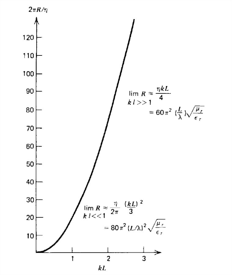
which is plotted versus \(kL\) in Fig. 9-14. This result can be checked in the limit as \(L\) becomes very small \(\left ( kL\ll 1 \right )\) since the radiation resistance should approach that of a point dipole given in Section 9-2-5. In this short dipole limit the bracketed terms in (14) are

\[ \lim_{kL\ll 1}\left\{\begin{matrix}
\displaystyle \frac{\sin kL}{kL}\approx 1-\frac{\left ( kL \right )^{2}}{6}\\ 
\displaystyle \cos kL\approx 1-\frac{\left (kL  \right )^{2}}{2}\\ 
\displaystyle kLSi\left ( kL \right )\approx \left ( kL \right )^{2}
\end{matrix}\right. \]

so that (14) reduces to

\[ \lim_{kL\ll 1}R\approx \frac{\eta }{2\pi }\frac{\left ( kL \right )^{2}}{3}=\frac{2\pi \eta }{3}\left ( \frac{L}{\lambda } \right )^{2}=80\pi ^{2}\left ( \frac{L}{\lambda } \right )^{2}\sqrt{\frac{\mu _{r}}{\varepsilon _{r}}} \]

which agrees with the results in Section 9-2-5. Note that for large dipoles \(\left ( kL\gg 1 \right )\), the sine integral term dominates with \(Si\left ( kL \right )\) approaching a constant value of \(\pi /2\) so that

\[ \lim_{kL\gg 1}R\approx \frac{\eta kL}{4}=60\sqrt{\frac{\mu _{r}}{\varepsilon _{r}}}\pi ^{2}\frac{L}{\lambda } \]