3.1: Two Phases

The two-phase system is the simplest of all polyphase systems to describe. Consider a pair of voltage sources sitting side by side with:

\[\ v_{1}=V \cos \omega t\label{1} \]

\(\ v_{2}=V \sin \omega t\label{2}\)

Suppose this system of sources is connected to al “balanced load”, as shown in Figure 1. To compute the power flows in the system, it is convenient to re-write the voltages in complex form:

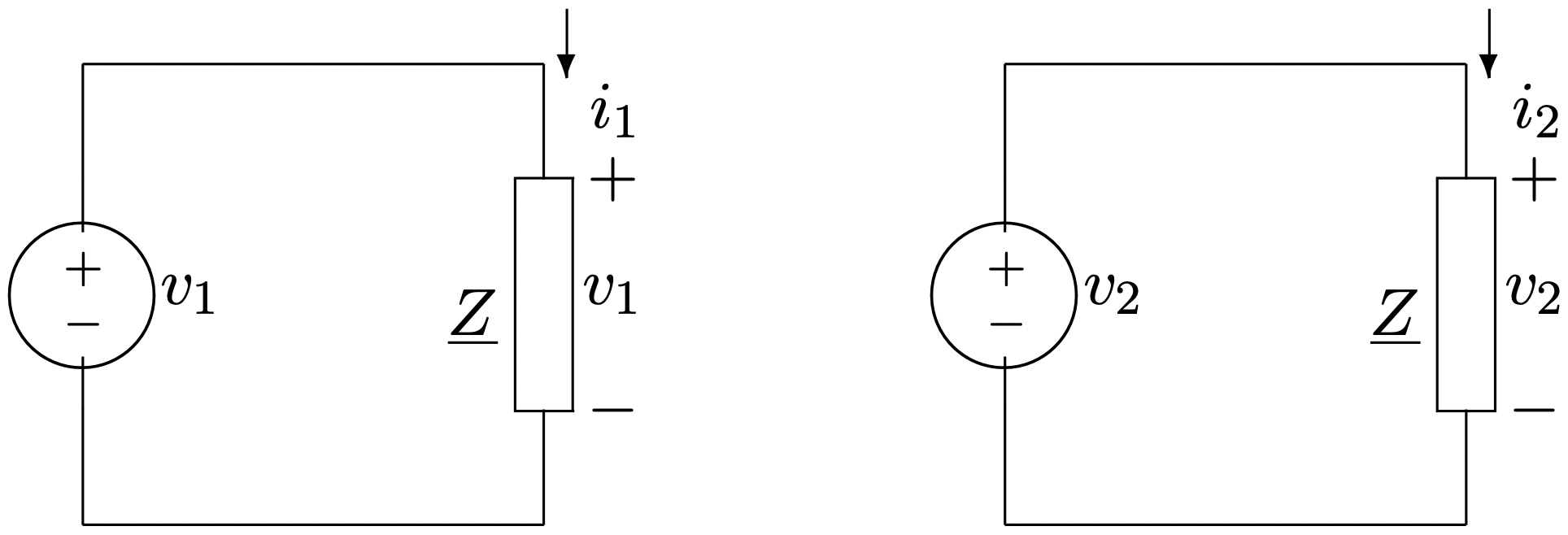Figure 1: Two-Phase System

\(\ v_{1}=R e\left[\underline{V} e^{j \omega t}\right]\label{3}\)

\(\ v_{2}=R e\left[-j \underline{V} e^{j \omega t}\right]\label{4}\)

\(\ ={Re}\left[\underline{V} e^{j\left(\omega t-\frac{\pi}{2}\right)}\right]\label{5}\)

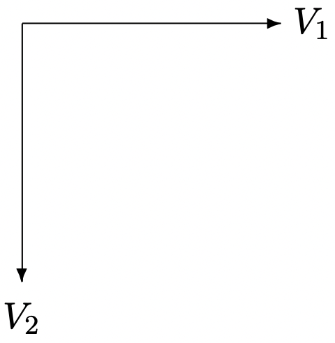Figure 2: Phasor Diagram for Two-Phase Source

If each source is connected to a load with impedance:

\(\ \underline{Z}=|\underline{Z}| e^{j \psi}\)

then the complex amplitudes of currents are:

\(\ \begin{array}{l}
\underline{I}_{1}=\frac{\underline{V}}{|\underline{Z}|} e^{-j \psi} \\
\underline{I}_{2}=\frac{\underline{V}}{|\underline{Z}|} e^{-j \psi} e^{-j \frac{\pi}{2}}
\end{array}\)

Each of the two phase networks has the same value for real and reactive power:

\(\ P+j Q=\frac{|\underline{V}|^{2}}{2|\underline{Z}|} e^{j \psi}\label{6}\)

or:

\(\ P=\frac{|\underline{V}|^{2}}{2|\underline{Z}|} \cos \psi\label{7}\)

\(\ Q=\frac{|\underline{V}|^{2}}{2|\underline{Z}|} \sin \psi\label{8}\)

The relationship between “complex power” and instantaneous power flow was worked out in Chapter 2 of these notes. For a system with voltage of the form:

\(\ v=R e\left[V e^{j \phi} e^{j \omega t}\right]\)

instantaneous power is given by:

\(\ p=P[1+\cos 2(\omega t+\phi)]+Q \sin 2(\omega t+\phi)\)

For the case under consideration here, \(\ \phi=0\) for phase 1 and \(\ \phi=-\frac{\pi}{2}\) for phase 2. Thus:

\(\ \begin{array}{l}
p_{1}=\frac{|\underline{V}|^{2}}{2|\underline{Z}|} \cos \psi[1+\cos 2 \omega t]+\frac{|\underline{V}|^{2}}{2|\underline{Z}|} \sin \psi \sin 2 \omega t \\
p_{2}=\frac{|\underline{V}|^{2}}{2|\underline{Z}|} \cos \psi[1+\cos (2 \omega t-\pi)]+\frac{|\underline{V}|^{2}}{2|\underline{Z}|} \sin \psi \sin (2 \omega t-\pi)
\end{array}\)

Note that the time-varying parts of these two expressions have opposite signs. Added together, they give instantaneous power:

\(\ p=p_{1}+p_{2}=\frac{|\underline{V}|^{2}}{|\underline{Z}|} \cos \psi\)

At least one of the advantages of polyphase power networks is now apparent. The use of a balanced polyphase system avoids the power flow pulsations due to ac voltage and current, and even the pulsations due to reactive energy flow. This has obvious benefits when dealing with motors and generators or, in fact, any type of source or load which would like to see constant power.