3.2: Three Phase Systems

Now consider the arrangement of three voltage sources illustrated in Figure 3.

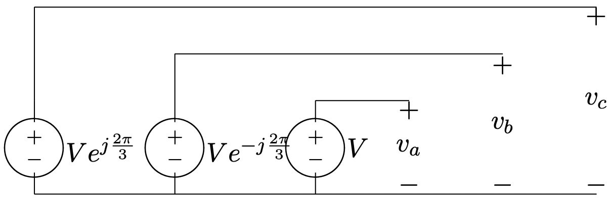Figure 3: Three- Phase Voltage Source

The three phase voltages are:

\[\ v_{a}=\quad V \cos \omega t \quad=R e\left[V e^{j \omega t}\right]\label{9} \]

\[\ v_{b}=V \cos \left(\omega t-\frac{2 \pi}{3}\right)=R e\left[V e^{j\left(\omega t-\frac{2 \pi}{3}\right)}\right]\label{10} \]

\[\ v_{c}=V \cos \left(\omega t+\frac{2 \pi}{3}\right)=\operatorname{Re}\left[V e^{j\left(\omega t+\frac{2 \pi}{3}\right)}\right]\label{11} \]

These three phase voltages are illustrated in the time domain in Figure 4 and as complex phasors in Figure 5. Note the symmetrical spacing in time of the voltages. As in earlier examples, the instantaneous voltages may be visualized by imagining Figure 5 spinning counterclockwise with angular velocity \(\ \omega\). The instantaneous voltages are just projections of the vectors of this “pinwheel” onto the horizontal axis.

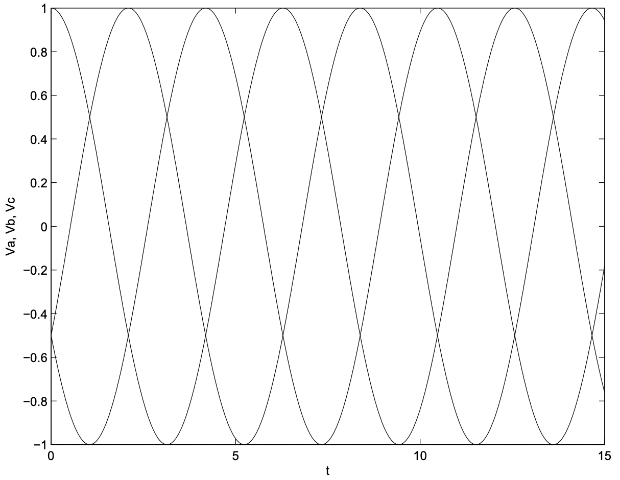Figure 4: Three Phase Voltages

Consider connecting these three voltage sources to three identical loads, each with complex impedance \(\ \underline{Z}\), as shown in Figure 6.

If voltages are as given by (9 - 11), then currents in the three phases are:

\[\ i_{a}=R e\left[\frac{\underline{\underline{V}}}{\underline{Z}} e^{j \omega t}\right]\label{12} \]

\[\ i_{b}=\operatorname{Re}\left[\frac{\underline{V}}{\underline{Z}} e^{j\left(\omega t-\frac{2 \pi}{3}\right)}\right]\label{13} \]

\[\ i_{c}=R e\left[\frac{\underline{V}}{\underline{Z}} e^{j\left(\omega t+\frac{2 \pi}{3}\right)}\right]\label{14} \]

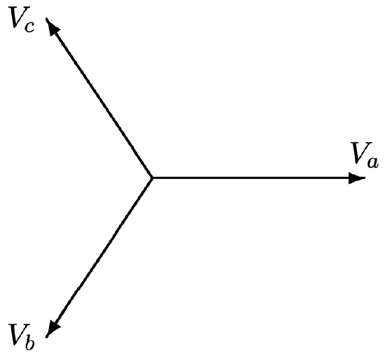Figure 5: Phasor Diagram: Three Phase Voltages

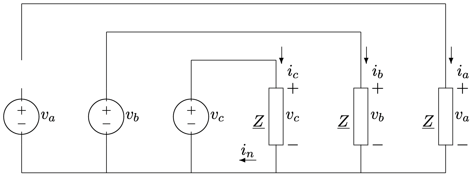Figure 6: Three- Phase Source Connected To Balanced Load

Complex power in each of the three phases is:

\[\ P+j Q=\frac{|\underline{V}|^{2}}{2|\underline{Z}|}(\cos \psi+j \sin \psi)\label{15} \]

Then, remembering the time phase of the three sources, it is possible to write the values of instantaneous power in the three phases:

\[\ p_{a}=\frac{|\underline{V}|^{2}}{2|\underline{Z}|}\{\cos \psi[1+\cos 2 \omega t]+\sin \psi \sin 2 \omega t\}\label{16} \]

\[\ p_{b}=\frac{|\underline{V}|^{2}}{2|\underline{Z}|}\left\{\cos \psi\left[1+\cos \left(2 \omega t-\frac{2 \pi}{3}\right)\right]+\sin \psi \sin \left(2 \omega t-\frac{2 \pi}{3}\right)\right\}\label{17} \]

\[\ p_{c}=\frac{|\underline{V}|^{2}}{2|\underline{Z}|}\left\{\cos \psi\left[1+\cos \left(2 \omega t+\frac{2 \pi}{3}\right)\right]+\sin \psi \sin \left(2 \omega t+\frac{2 \pi}{3}\right)\right\}\label{18} \]

The sum of these three expressions is total instantaneous power, which is constant:

\[\ p=p_{a}+p_{b}+p_{c}=\frac{3}{2} \frac{|\underline{V}|^{2}}{|\underline{Z}|} \cos \psi\label{19} \]

It is useful, in dealing with three phase systems, to remember that

\(\ \cos x+\cos \left(x-\frac{2 \pi}{3}\right)+\cos \left(x+\frac{2 \pi}{3}\right)=0\)

regardless of the value of \(\ x\).

Now consider the current in the neutral wire, \(\ i_{n}\) in Figure 6. This current is given by:

\[\ i_{n}=i_{a}+i_{b}+i_{c}=R e\left[\frac{V}{\underline{Z}}\left(e^{j \omega t}+e^{j\left(\omega t-\frac{2 \pi}{3}\right)}+e^{j\left(\omega t+\frac{2 \pi}{3}\right)}\right)\right]=0\label{20} \]

This shows the most important advantage of three-phase systems over two-phase systems: a wire with no current in it does not have to be very large. In fact, the neutral connection may be eliminated completely in many cases. The network shown in Figure 7 will work as well as the network in Figure 6 in most cases in which the voltages and load impedances are balanced.

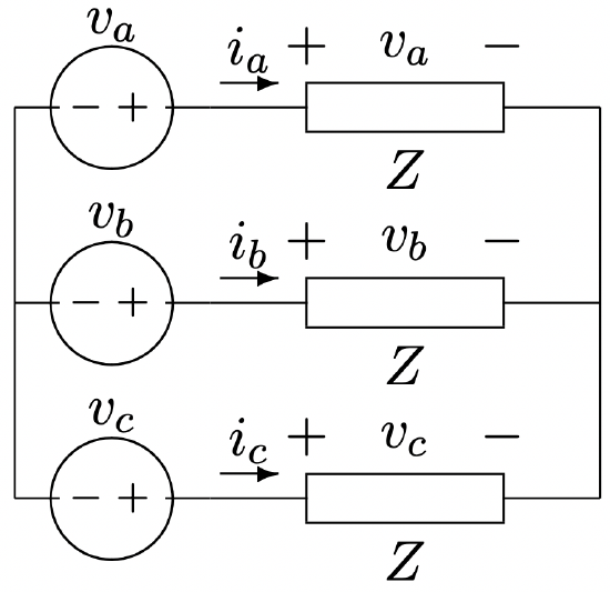Figure 7: Ungrounded Three-Phase Source and Load

There is a fundamental difference between grounded and undgrounded systems if perfectly balanced conditions are not maintained. In effect, the ground wire provides isolation between the phases by fixing the neutral voltage a the star point to be zero. If the load impedances are not equal the load is said to be unbalanced. If the system is grounded there will be current in the neutral. If an unbalanced load is not grounded, the star point voltage will not be zero, and the voltages will be different in the three phases at the load, even if the voltage sources all have the same magnitude.