3.3: Line-Line Voltages

A balanced three-phase set of voltages has a well defined set of line-line voltages. If the line-toneutral voltages are given by (9 - 11), then line-line voltages are:

\[\ v_{a b}=v_{a}-v_{b}=\operatorname{Re}\left[\underline{V}\left(1-e^{-j \frac{2 \pi}{3}}\right) e^{j \omega t}\right]\label{21} \]

\[\ v_{b c}=v_{b}-v_{c}=\operatorname{Re}\left[\underline{V}\left(e^{-j \frac{2 \pi}{3}}-e^{j \frac{2 \pi}{3}}\right) e^{j \omega t}\right]\label{22} \]

\[\ v_{c a}=v_{c}-v_{a}=R e\left[\underline{V}\left(e^{j \frac{2 \pi}{3}}-1\right) e^{j \omega t}\right]\label{23} \]

and these reduce to:

\[\ v_{a b}=\operatorname{Re}\left[\sqrt{3} \underline{V} e^{j \frac{\pi}{6}} e^{j \omega t}\right]\label{24} \]

\[\ v_{b c}=R e\left[\sqrt{3} \underline{V} e^{-j \frac{\pi}{2}} e^{j \omega t}\right]\label{25} \]

\[\ v_{c a}=\operatorname{Re}\left[\sqrt{3} \underline{V} e^{j \frac{5 \pi}{6}} e^{j \omega t}\right]\label{26} \]

The phasor relationship of line-to-neutral and line-to-line voltages is shown in Figure 8. Two things should be noted about this relationship:

• The line-to-line voltage set has a magnitude that is larger than the line-ground voltage by a factor of \(\ \sqrt{3}\).
• Line-to-line voltages are phase shifted by 30^o ahead of line-to-neutral voltages.

Clearly, line-to-line voltages themselves form a three-phase set just as do line-to-neutral voltages. Power system components (sources, transformer windings, loads, etc.) may be connected either between lines and neutral or between lines. The former connection of often called wye, the latter is called delta, for obvious reasons.

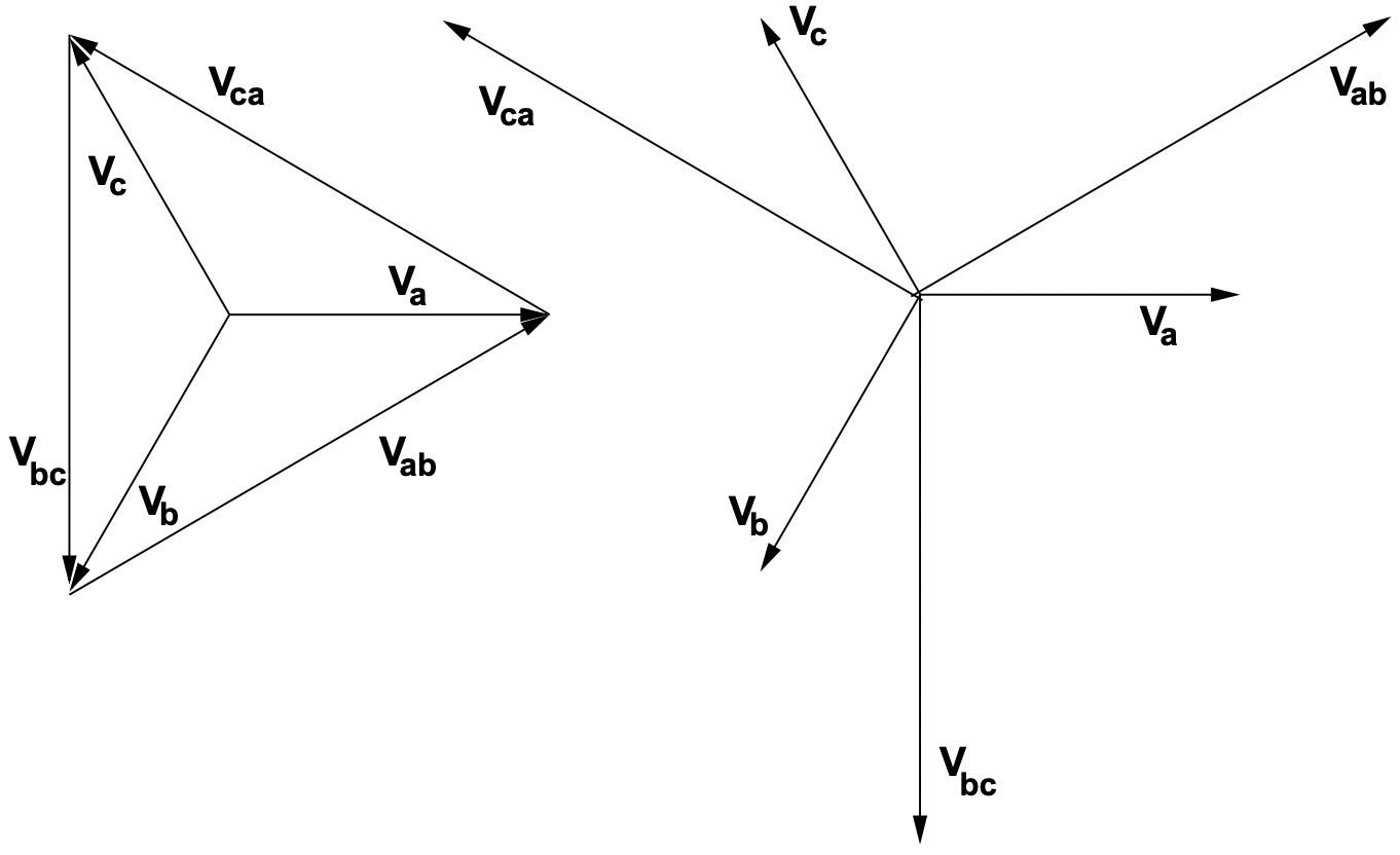Figure 8: Line-Neutral and Line-Line Voltages

It should be noted that the wye connection is at least potentially a four-terminal connection, while the delta connection is inherently three-terminal. The difference is the availability of a neutral point. Under balanced operating conditions this is unimportant, but the difference is apparent and important under unbalanced conditions.

Example: Wye and Delta Connected Loads

Loads may be connected in either line-to-neutral or line-to-line configuration. An example of the use of this flexibility is in a fairly commonly used distribution system with a line-to-neutral voltage of 120 V, RMS. In this system the line-to-line voltage is 208 V, RMS. Single phase loads may be connected either line-to-line or line-to-neutral.

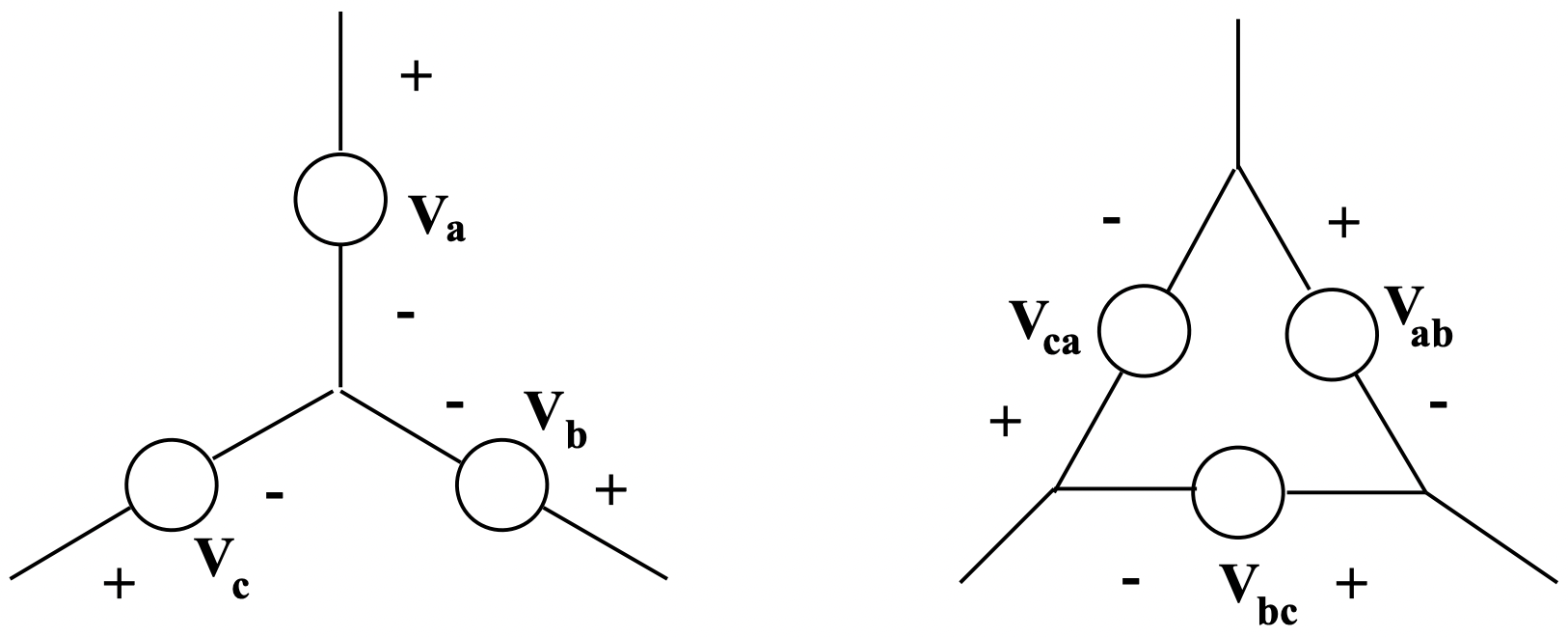Figure 9: Wye And Delta Connected Voltage Sources

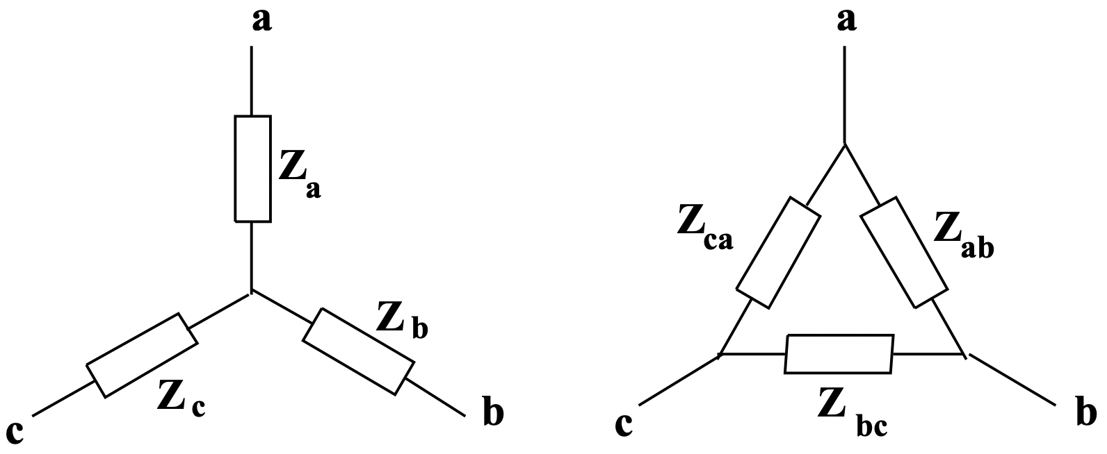Figure 10: Wye And Delta Connected Impedances

Suppose it is necessary to build a resistive heater to deliver 6 kW, to be made of three elements which may be connected in either wye or delta. Each of the three elements must dissipate 2000 W.

Thus, since \(\ P=\frac{V^{2}}{R}\), the wye connected resistors would be:

\(\ R_{y}=\frac{120^{2}}{2000}=7.2 \Omega\)

while the delta connected resistors would be:

\(\ R_{\Delta}=\frac{208^{2}}{2000}=21.6 \Omega\)

As is suggested by this example, wye and delta connected impedances are often directly equivalent. In fact, ungrounded connections are three-terminal networks which may be represented in two ways. The two networks shown in Figure 10, combinations of three passive impedances, are directly equivalent and identical in their terminal behavior if the relationships between elements are as given in (27 - 32).

\[\ \underline{Z}_{a b}=\frac{\underline{Z}_{a} \underline{Z}_{b}+\underline{Z}_{b} \underline{Z}_{c}+\underline{Z}_{c} \underline{Z}_{a}}{\underline{Z}_{c}}\label{27} \]

\[\ \underline{Z}_{b c}=\frac{\underline{Z}_{a} \underline{Z}_{b}+\underline{Z}_{b} \underline{Z}_{c}+\underline{Z}_{c} \underline{Z}_{a}}{\underline{Z}_{a}}\label{28} \]

\[\ \underline{Z}_{c a}=\frac{\underline{Z}_{a} \underline{Z}_{b}+\underline{Z}_{b} \underline{Z}_{c}+\underline{Z}_{c} \underline{Z}_{a}}{\underline{Z}_{b}}\label{29} \]

\[\ \underline{Z}_{a}=\frac{\underline{Z}_{a b} \underline{Z}_{c a}}{\underline{Z}_{a b}+\underline{Z}_{b c}+\underline{Z}_{c a}}\label{30} \]

\[\ \underline{Z}_{b}=\frac{\underline{Z}_{a b} \underline{Z}_{b c}}{\underline{Z}_{a b}+\underline{Z}_{b c}+\underline{Z}_{c a}}\label{31} \]

\[\ \underline{Z}_{c}=\frac{\underline{Z}_{b c} \underline{Z}_{c a}}{\underline{Z}_{a b}+\underline{Z}_{b c}+\underline{Z}_{c a}}\label{32} \]

A special case of the wye-delta equivalence is that of balanced loads, in which:

\(\ \underline{Z}_{a}=\underline{Z}_{b}=\underline{Z}_{c}=\underline{Z}_{y}\)

and

\(\ \underline{Z}_{a b}=\underline{Z}_{b c}=\underline{Z}_{c a}=\underline{Z}_{\Delta}\)

in which case:

\(\ \underline{Z}_{\Delta}=3 \underline{Z}_{y}\)

Example: Use of Wye-Delta for Unbalanced Loads

The unbalanced load shown in Figure 11 is connected to a balanced voltage source. The problem is to determine the line currents. Note that his load is ungrounded (if it were grounded, this would be a trivial problem). The voltages are given by:

\(\ \begin{array}{l}
v_{a}=V \cos \omega t \\
v_{b}=V \cos \left(\omega t-\frac{2 \pi}{3}\right) \\
v_{c}=V \cos \left(\omega t+\frac{2 \pi}{3}\right)
\end{array}\)

To solve this problem, convert both the source and load to delta equivalent connections, as shown in Figure 12. The values of the three resistors are:

\(\ \begin{array}{c}
r_{a b}=r_{c a}=\frac{2+4+2}{2}=4 \\
r_{b c}=\frac{2+4+2}{1}=8
\end{array}\)

The complex amplitudes of the equivalent voltage sources are:

\(\ \begin{array}{ll}
\underline{V}_{a b}&= \underline{V}_{a}-\underline{V}_{b}=\underline{V}\left(1-e^{-j \frac{2 \pi}{3}}\right)&= \underline{V} \sqrt{3} e^{j \frac{\pi}{6}} \\
\underline{V}_{b c}&=\underline{V}_{b}-\underline{V}_{c}=\underline{V}\left(e^{-j \frac{2 \pi}{3}}-e^{j \frac{2 \pi}{3}}\right)&= \underline{V} \sqrt{3} e^{-j \frac{\pi}{2}} \\
\underline{V}_{c a}&=\underline{V}_{c}-\underline{V}_{a}=\underline{V}\left(e^{j \frac{2 \pi}{3}}-1\right)&= \underline{V} \sqrt{3} e^{j \frac{5 \pi}{6}}
\end{array}\)

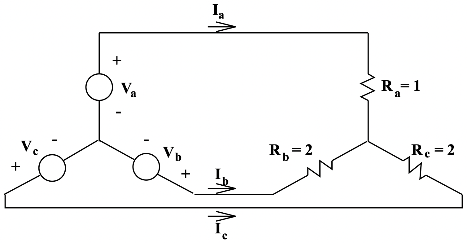Figure 11: Unbalanced Load

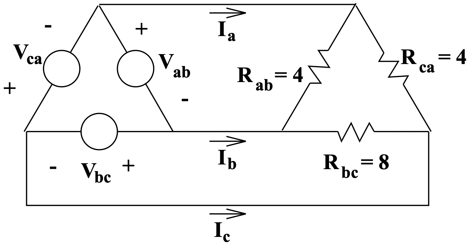Figure 12: Delta Equivalent

Currents in each of the equivalent resistors are:

\(\ \underline{I}_{1}=\frac{\underline{V}_{a b}}{r_{a b}} \quad \underline{I}_{2}=\frac{\underline{V}_{b c}}{r_{b c}} \quad \underline{I}_{3}=\frac{V_{c a}}{r_{c a}}\)

The line curents are then just the difference between current in the legs of the delta:

\(\ \begin{array}{l}
I_{a}=I_{1}-I_{3}=\sqrt{3} V\left(\frac{e^{j \frac{\pi}{6}}}{4}-\frac{e^{j \frac{5 \pi}{6}}}{4}\right)=\frac{3}{4} V \\
I_{b}=I_{2}-I_{1}=\sqrt{3} V\left(\frac{e^{-j \frac{\pi}{2}}}{8}-\frac{e^{j} \frac{\pi}{6}}{4}\right)=-\left(\frac{3}{8}+j \frac{1}{4}\right) V \\
I_{c}=I_{3}-I_{2}=\sqrt{3} V\left(\frac{e^{5 \frac{5 \pi}{6}}}{4}-\frac{e^{-j \frac{\pi}{2}}}{8}\right)=-\left(\frac{3}{8}-j \frac{1}{4}\right) V
\end{array}\)

These are shown in Figure 13.

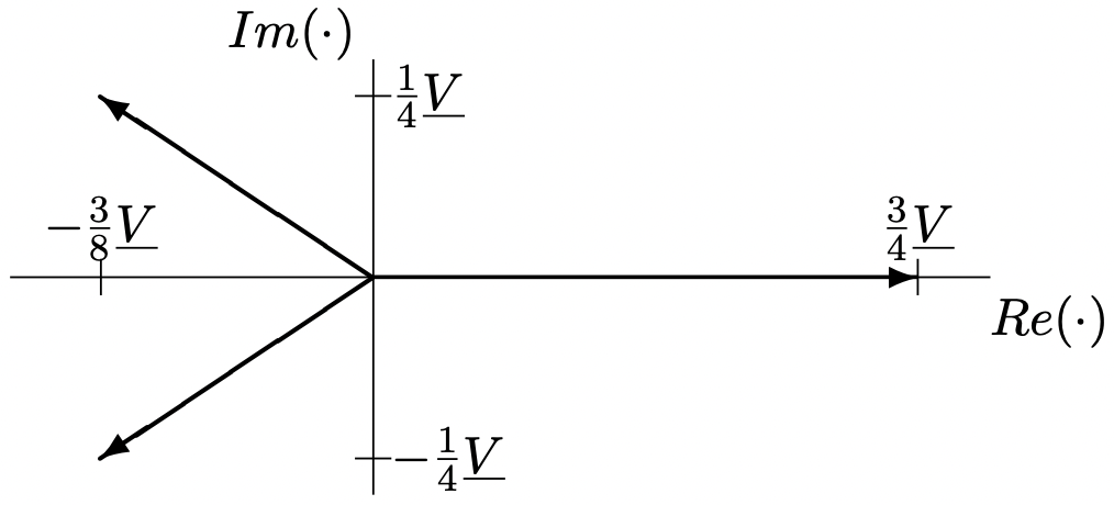Figure 13: Line Currents