3.7: Introduction To Per-Unit Systems

Strictly speaking, per-unit systems are nothing more than normalizations of voltage, current, impedance and power. These normalizations of system parameters because they provide simplifications in many network calculations. As we will discover, while certain ordinary parameters have very wide ranges of value, the equivalent per-unit parameters fall in a much narrower range. This helps in understanding how certain types of system behave.

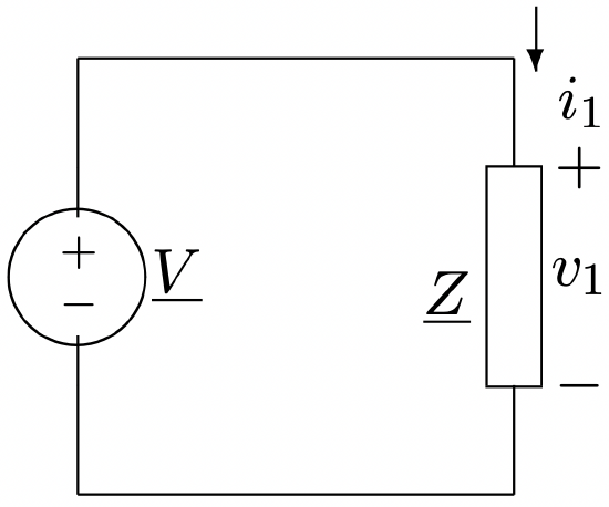Figure 22: Example

Normalization Of Voltage And Current

The basis for the per-unit system of notation is the expression of voltage and current as fractions of base levels. Thus the first step in setting up a per-unit normalization is to pick base voltage and current.

Consider the simple situation shown in Figure 22. For this network, the complex amplitudes of voltage and current are:

\[\ \underline{V}=\underline{I Z}\label{48} \]

We start by defining two base quantities, \(\ V_B\) for voltage and \(\ I_B\) for current. In many cases, these will be chosen to be nominal or rated values. For generating plants, for example, it is common to use the rated voltage and rated current of the generator as base quantities. In other situations, such as system stability studies, it is common to use a standard, system wide base system.

The per-unit voltage and current are then simply:

\[\ \underline{v}=\frac{\underline{V}}{V_{B}}\label{49} \]

\[\ \underline{i}=\frac{I}{I_{B}}\label{50} \]

Applying (49) and (50) to (48), we find:

\[\ \underline{v}=\underline{i z}\label{51} \]

where the per-unit impedance is:

\[\ \underline{z}=\underline{Z} \frac{I_{B}}{V_{B}}\label{52} \]

This leads to a definition for a base impedance for the system:

\[\ Z_{B}=\frac{V_{B}}{I_{B}}\label{53} \]

Of course there is also a base power, which for a single phase system is:

\[\ P_{B}=V_{B} I_{B}\label{54} \]

as long as \(\ V_B\) and \(\ I_B\) are expressed in RMS. It is interesting to note that, as long as normalization is carried out in a consistent way, there is no ambiguity in per-unit notation. That is, peak quantities normalized to peak base quantities will be the same, in per-unit, as RMS quantities normalized to RMS bases. This advantage is even more striking in polyphase systems, as we are about to see.

Three Phase Systems

When describing polyphase systems, we have the choice of using either line-line or line-neutral voltage and line current or current in delta equivalent loads. In order to keep straight analysis in ordinary variable, it is necessary to carry along information about which of these quantities is being used. There is no such problem with per-unit notation.

We may use as base quantities either line to neutral voltage \(\ V_{B l-g}\) or line to line voltage \(\ V_{B l-l}\).

Taking the base current to be line current \(\ I_{B l}\), we may express base power as:

\[\ P_{B}=3 V_{B l-g} I_{B l}\label{55} \]

Because line-line voltage is, under normal operation, \(\ \sqrt{3}\) times line-neutral voltage, an equivalent statement is:

\[\ P_{B}=\sqrt{3} V_{B l-l} I_{B l}\label{56} \]

If base impedance is expressed by line-neutral voltage and line current (This is the common convention, but is not required),

\[\ Z_{B}=\frac{V_{B l-g}}{I_{B l}}\label{57} \]

Then, base impedance is, written in terms of base power:

\[\ Z_{B}=\frac{P_{B}}{3 I_{B}^{2}}=3 \frac{V_{B l-g}^{2}}{P_{B}}=\frac{V_{B l-l}^{2}}{P_{B}}\label{58} \]

Note that a single per-unit voltage applied equally well to line-line, line-neutral, peak and RMS quantities. For a given situation, each of these quantities will have a different ordinary value, but there is only one per-unit value.

Networks With Transformers

One of the most important advantages of the use of per-unit systems arises in the analysis of networks with transformers. Properly applied, a per-unit normalization will cause nearly all ideal transformers to dissapear from the per-unit network, thus greatly simplifying analysis.

To show how this comes about, consider the ideal transformer as shown in Figure 23. The

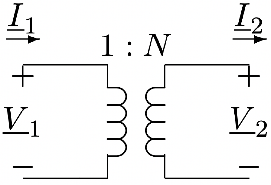Figure 23: Ideal Transformer With Voltage And Current Conventions Noted

ideal transformer imposes the constraints that:

\(\ \begin{array}{l}
\underline{V}_{2}=N \underline{V}_{1} \\
\underline{I}_{2}=\frac{1}{N} \underline{I}_{1}
\end{array}\)

Normalized to base quantities on the two sides of the transformer, the per-unit voltage and current are:

\(\ \begin{array}{l}
\underline{v}_{1}=\frac{\underline{V}_{1}}{V_{B 1}} \\
\underline{i}_{1}=\frac{\underline{I}_{1}}{I_{B 1}} \\
\underline{v}_{2}=\frac{\underline{V}_{2}}{V_{B 2}} \\
\underline{i}_{2}=\frac{\underline{I}_{2}}{I_{B 2}}
\end{array}\)

Now: note that if the base quantities are related to each other as if they had been processed by the transformer:

\[\ V_{B 2}=N V_{B 1}\label{59} \]

\[\ I_{B 2}=\frac{I_{B 1}}{N}\label{60} \]

then \(\ \underline{v}_{1}=\underline{v}_{2}\) and \(\ \underline{i}_{1}=\underline{i}_{2}\), as if the ideal transformer were not there (that is, consisted of an ideal wire).

Expressions (59) and (60) reflect a general rule in setting up per-unit normalizations for systems with transformers. Each segment of the system should have the same base power. Base voltages transform according to transformer voltage ratios. For three-phase systems, of course, the voltage ratios may differ from the physical turns ratios by a factor of \(\ \sqrt{3}\) if delta-wye or wye-delta connections are used. It is, however, the voltage ratio that must be used in setting base voltages.

Transforming From One Base To Another

Very often data such as transformer leakage inductance is given in per-unit terms, on some base (perhaps the units rating), while in order to do a system study it is necessary to express the same data in per-unit in some other base (perhaps a unified system base). It is always possible to do this by the two step process of converting the per-unit data to its ordinary form, then re-normalizing it in the new base. However, it is easier to just convert it to the new base in the following way.

Note that impedance in Ohms (ordinary units) is given by:

\[\ \underline{Z}=\underline{z}_{1} Z_{B 1}=\underline{z}_{2} Z_{B 2}\label{61} \]

Here, of course, \(\ \underline{z}_{1}\) and \(\ \underline{z}_{2}\) are the same per-unit impedance expressed in different bases. This could be written as:

\[\ \underline{z}_{1} \frac{V_{B 1}^{2}}{P_{B 1}}=\underline{z}_{2} \frac{V_{B 2}^{2}}{P_{B 2}}\label{62} \]

This yields a convenient rule for converting from one base system to another:

\[\ \underline{z}_{1}=\frac{P_{B 1}}{P_{B 2}}\left(\frac{V_{B 2}}{V_{B 1}}\right)^{2} \underline{z}_{2}\label{63} \]

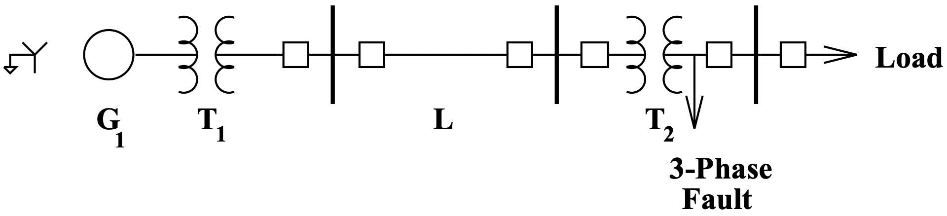Figure 24: One-Line Diagram Of Faulted System

Example: Fault Study

To illustrate some of the concepts with which we have been dealing, we will do a short circuit analysis of a simple power system. This system is illustrated, in one-line diagram form, in Figure 24.

A one-line diagram is a way of conveying a lot of information about a power system without becoming cluttered with repetitive pieces of data. Drawing all three phases of a system would involve quite a lot of repetition that is not needed for most studies. Further, the three phases can be re-constructed from the one-line diagram if necessary. It is usual to use special symbols for different components of the network. For our network, we have the following pieces of data:

Symbol	Component	Base P	Base V	Impedance
\(\ G_{1}\)	Generator	200	13.8	\(\ j .18\)
\(\ T_{1}\)	Transformer	200	13.8/138	\(\ j .12\)
\(\ L_{1}\)	Trans. Line	100	138	\(\ .02+j .05\)
\(\ T_{2}\)	Transformer	50	138/34.5	\(\ j .08\)

A three-phase fault is assumed to occur on the 34.5 kV side of the transformer \(\ T_{2}\). This is a symmetrical situation, so that only one phase must be represented. The per-unit impedance diagram is shown in Figure 25. It is necessary to proceed now to determine the value of the components in this circuit.

Figure 25: Impedance Diagram For Fault Example

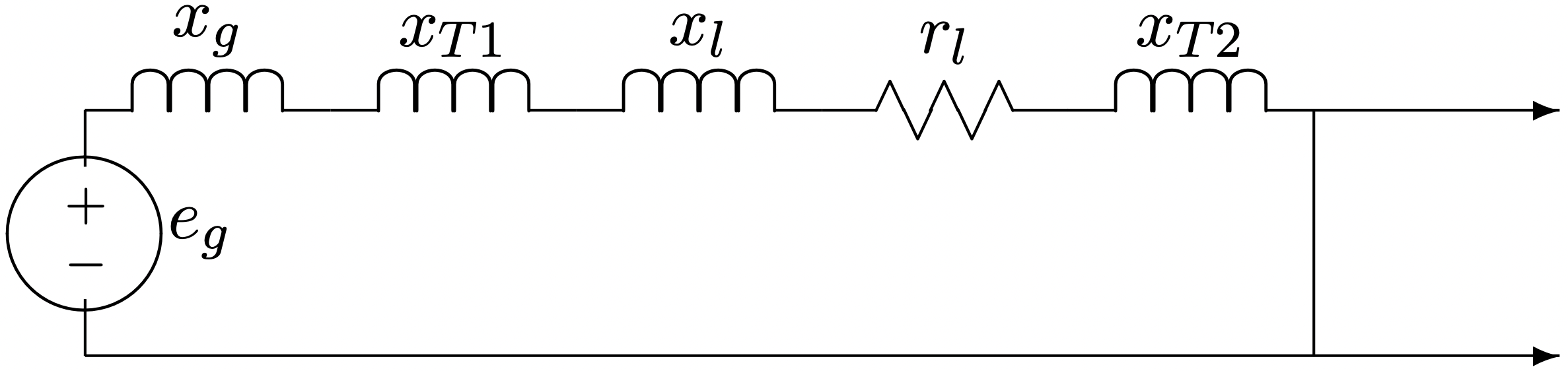
First, it is necessary to establish a uniform base an per-unit value for each of the system components. Somewhat arbitrarily, we choose as the base segment the transmission line. Thus all of the parameters must be put into a base power of 100 MVA and voltage bases of 138 kV on the line, 13.8 kV at the generator, and 34.5 kV at the fault. Using (62):

\(\ \begin{aligned}
x_{g}&=\frac{100}{200} \times .18 &=.09 \text { per-unit } \\
x_{T 1}&=\frac{100}{200} \times .12 &=.06 \text { per-unit } \\
x_{T 2}&=\frac{100}{50} \times .08 &=.16 \text { per-unit } \\
r_{l}&=&.02 \text { per-unit } \\
x_{l}&=&.05 \text { per-unit }
\end{aligned}\)

Total impedance is:

\(\ \begin{aligned}
\underline{z} &=j\left(x_{g}+x_{T 1}+x_{l}+x_{T 2}\right)+r_{l} \\
&=j .36+.02 \text { per-unit } \\
|\underline{z}| &=.361 \text { per-unit }
\end{aligned}\)

Now, if \(\ e_{g}\) is equal to one per-unit (generator internal voltage equal to base voltage), then the per-unit current is:

\(\ |\underline{i}|=\frac{1}{.361}=.277 \text { per-unit }\)

This may be translated back into ordinary units by getting base current levels. These are:

• \(\ I_{B}=\frac{100 \mathrm{MVA}}{\sqrt{3} \times 13.8 \mathrm{kV}}=4.18 \mathrm{kA}\)
• \(\ I_{B}=\frac{100 \mathrm{MVA}}{\sqrt{3} \times 138 \mathrm{kV}}=418 \mathrm{~A}\)
• \(\ I_{B}=\frac{100 \mathrm{MVA}}{\sqrt{3} \times 34.5 \mathrm{kV}}=1.67 \mathrm{kA}\)

Then the actual fault currents are:

• At the generator \(\ \left|\underline{I}_{f}\right|=11,595 \mathrm{~A}\)
• On the transmission line \(\ \left|\underline{I}_{f}\right|=1159 \mathrm{~A}\)
• At the fault \(\ \left|\underline{I}_{f}\right|=4633 \mathrm{~A}\)