3.6: Polyphase Lines and Single-Phase Equivalents

By now, one might suspect that a balanced polyphase system may be regarded simply as three single-phase systems, even though the three phases are physically interconnected. This feeling is reinforced by the equivalence between \( wye\) and \( delta\) connected sources and impedances. One more step is required to show that single phase equivalence is indeed useful, and this concerns situations in which the phases have mutual coupling.

In speaking of lines, we mean such system elements as transmission or distribution lines: overhead wires, cables or even in-plant buswork. Such elements have impedance, so that there is some voltage drop between the sending and receiving ends of the line. This impedance is more than just conductor resistance: the conductors have both self and mutual inductance, because currents in the conductors make magnetic flux which, in turn, is linked by all conductors of the line.

A schematic view of a line is shown in Figure 20. Actually, only the inductance components of line impedance are shown, since they are the most interesting parts of line impedance. Working in complex amplitudes, it is possible to write the voltage drops for the three phases by:

\[\ \underline{V}_{a 1}-\underline{V}_{a 2}=j \omega L \underline{I}_{a}+j \omega M\left(\underline{I}_{b}+\underline{I}_{c}\right)\label{43} \]

\[\ \underline{V}_{b 1}-\underline{V}_{b 2}=j \omega L \underline{I}_{b}+j \omega M\left(\underline{I}_{a}+\underline{I}_{c}\right)\label{44} \]

\[\ \underline{V}_{c 1}-\underline{V}_{c 2}=j \omega L \underline{I}_{c}+j \omega M\left(\underline{I}_{a}+\underline{I}_{b}\right)\label{45} \]

If the currents form a balanced set:

\[\ \underline{I}_{a}+\underline{I}_{b}+\underline{I}_{c}=0\label{46} \]

Then the voltage drops are simply:

\( \begin{array}{l}
\underline{V}_{a 1}-\underline{V}_{a 2}=j \omega(L-M) \underline{I}_{a} \\
\underline{V}_{b 1}-\underline{V}_{b 2}=j \omega(L-M) \underline{I}_{b} \\
\underline{V}_{c 1}-\underline{V}_{c 2}=j \omega(L-M) \underline{I}_{c}
\end{array}\)

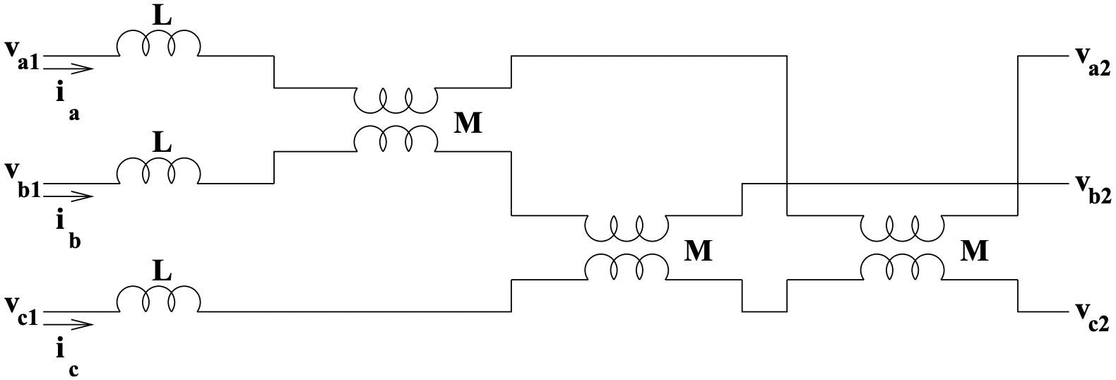Figure 20: Schematic Of A Balanced Three-Phase Line With Mutual Coupling

In this case, an apparent inductance, suitable for the balanced case, has been defined:

\[\ L_{1}=L-M\label{47} \]

which describes the behavior of one phase in terms of its own current. It is most important to note that this inductance is a valid description of the line only if (46) holds, which it does, of course, in the balanced case.

Example

To show how the analytical techniques which come from the network simplification resulting from single phase equivalents and wye-delta transformations, consider the following problem:

A three-phase resistive load is connected to a balanced three-phase source through a transformer connected in delta-wye and a polyphase line, as shown in Figure 21.

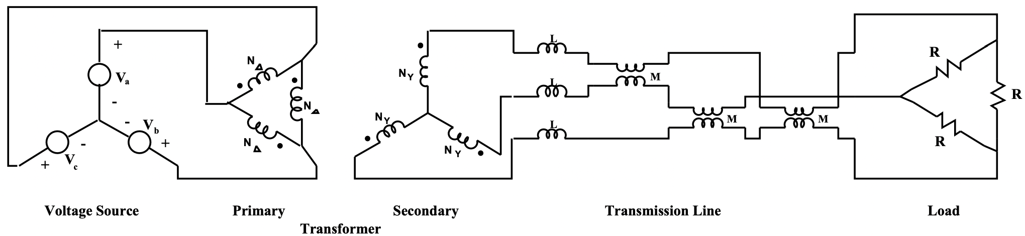Figure 21: Example

The problem is to calculate power dissipated in the load resistors. The three- phase voltage source has:

\( \begin{aligned}
v_{a} &=\operatorname{Re}\left[\sqrt{2} V_{R M S} e^{j \omega t}\right] \\
v_{b} &=\operatorname{Re}\left[\sqrt{2} V_{R M S} e^{j\left(\omega t-\frac{2 \pi}{3}\right)}\right] \\
v_{c} &=\operatorname{Re}\left[\sqrt{2} V_{R M S} e^{j\left(\omega t+\frac{2 \pi}{3}\right)}\right]
\end{aligned}\)

This problem is worked by a succession of simple transformations. First, the delta connected resistive load is converted to its equivalent \( wye\) with \( R_{Y}=\frac{R}{3}\).

Next, since the problem is balanced, the self- and mutual inductances of the line are directly equivalent to self inductances in each phase of \( L_{1}=L-M\).

Now, the transformer secondary is facing an impedance in each phase of:

\( \underline{Z}_{Y s}=j \omega L_{1}+R_{Y}\)

The delta-wye transformer has a voltage ratio of:

\( \frac{v_{p}}{v_{s}}=\frac{N_{\Delta}}{\sqrt{3} N_{Y}}\)

so that, on the primary side of the transformer, the line and load impedance is:

\( \underline{Z}_{p}=j \omega L_{e q}+R_{e q}\)

where the equivalent elements are:

\( \begin{aligned}
L_{e q} &=\frac{1}{3}\left(\frac{N_{\Delta}}{N_{Y}}\right)^{2}(L-M) \\
R_{e q} &=\frac{1}{3}\left(\frac{N_{\Delta}}{N_{Y}}\right)^{2} \frac{R}{3}
\end{aligned}\)

Magnitude of current flowing in each phase of the source is:

\( |\underline{I}|=\frac{\sqrt{2} V_{R M S}}{\sqrt{\left(\omega L_{e q}\right)^{2}+R_{e q}^{2}}}\)

Dissipation in one phase is:

\[ \begin{aligned}
P_{1} &=\frac{1}{2}|\underline{I}|^{2} R_{e q} \\
&=\frac{V_{R M S}^{2} R_{e q}}{\left(\omega L_{e q}\right)^{2}+R_{e q}^{2}}
\end{aligned}\]

And, of course, total power dissipated is just three times the single phase dissipation.