
4.1: The Symmetrical Component Transformation
- Page ID
- 55550

The basis for this analytical technique is a transformation of the three voltages and three currents into a second set of voltages and currents. This second set is known as the symmetrical components.
Working in complex amplitudes:
\[\ v_{a}=\operatorname{Re}\left(\underline{V}_{a} e^{j \omega t}\right)\label{1} \]
\[\ v_{b}=\operatorname{Re}\left(\underline{V}_{b} e^{j\left(\omega t-\frac{2 \pi}{3}\right)}\right)\label{2} \]
\[\ v_{c}=\operatorname{Re}\left(\underline{V}_{c} e^{j\left(\omega t+\frac{2 \pi}{3}\right)}\right)\label{3} \]
The transformation is defined as:
\[\ \left[\begin{array}{l}
\underline{V}_{1} \\
\underline{V}_{2} \\
\underline{V}_{0}
\end{array}\right]=\frac{1}{3}\left[\begin{array}{lll}
1 & \underline{a} & \underline{a}^{2} \\
1 & \underline{a}^{2} & \underline{a} \\
1 & 1 & 1
\end{array}\right]\left[\begin{array}{l}\label{4}
\underline{V}_{a} \\
\underline{V}_{b} \\
\underline{V}_{c}
\end{array}\right] \nonumber \]
where the complex number \(\ \underline{a}\) is:
\[\ \underline{a} \quad=e^{j \frac{2 \pi}{3}} \quad=-\frac{1}{2}+j \frac{\sqrt{3}}{2}\label{5} \]
\[\ \underline{a}^{2}=e^{j \frac{4 \pi}{3}}=e^{-j \frac{2 \pi}{3}}=-\frac{1}{2}-j \frac{\sqrt{3}}{2}\label{6} \]
\[\ \underline{a}^{3} \quad=1\label{7} \]
This transformation may be used for both voltage and current, and works for variables in ordinary form as well as variables that have been normalized and are in per-unit form. The inverse of this transformation is:
\[\ \left[\begin{array}{l}
\underline{V}_{a} \\
\underline{V}_{b} \\
\underline{V}_{c}
\end{array}\right]=\left[\begin{array}{lll}
1 & 1 & 1 \\
\underline{a}^{2} & \underline{a} & 1 \\
\underline{a} & \underline{a}^{2} & 1
\end{array}\right]\left[\begin{array}{l}
\underline{V}_{1} \\
\underline{V}_{2} \\
\underline{V}_{0}
\end{array}\right]\label{8} \]
The three component variables \(\ \underline{V}_{1}\), \(\ \underline{V}_{2}\), \(\ \underline{V}_{0}\) are called, respectively, positive sequence, negative sequence and zero sequence. They are called symmetrical components because, taken separately, they transform into symmetrical sets of voltages. The properties of these components can be demonstrated by tranforming each one back into phase variables.
Consider first the positive sequence component taken by itself:
\[\ \underline{V}_{1}=V\label{9} \]
\[\ \underline{V}_{2}=0\label{10} \]
\[\ \underline{V}_{0}=0\label{11} \]
yields:
\[\ \underline{V}_{a}=V \quad \text { or } \quad v_{a}=V \cos \omega t\label{12} \]
\[\ \underline{V}_{b}=\underline{a}^{2} V \quad \text { or } \quad v_{b}=V \cos \left(\omega t-\frac{2 \pi}{3}\right)\label{13} \]
\[\ \underline{V}_{c}=\underline{a} V \quad \text { or } \quad v_{c}=V \cos \left(\omega t+\frac{2 \pi}{3}\right)\label{14} \]
This is the familiar balanced set of voltages: Phase b lags phase a by 120o phase c lags phase b and phase a lags phase c.
The same transformation carried out on a negative sequence voltage:
\[\ \underline{V}_{1}=0\label{15} \]
\[\ \underline{V}_{2}=V\label{16} \]
\[\ \underline{V}_{0}=0\label{17} \]
yields:
\[\ \underline{V}_{a}=V \quad \text { or } \quad v_{a}=V \cos \omega t\label{18} \]
\[\ \underline{V}_{b}=\underline{a} V \quad \text { or } \quad v_{b}=V \cos \left(\omega t+\frac{2 \pi}{3}\right)\label{19} \]
\[\ \underline{V}_{c}=\underline{a}^{2} V \quad \text { or } \quad v_{c}=V \cos \left(\omega t-\frac{2 \pi}{3}\right)\label{20} \]
This is called negative sequence because the sequence of voltages is reversed: phase b now leads phase a rather than lagging. Note that the negative sequence set is still balanced in the sense that the phase components still have the same magnitude and are separated by 120o . The only difference between positive and negative sequence is the phase rotation. This is shown in Figure 1.
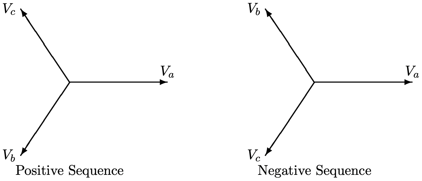 Figure 1: Phasor Diagram: Three Phase Voltages
The third symmetrical component is zero sequence. If:
\[\ \underline{V}_{1}=0\label{21} \]
\[\ \underline{V}_{2}=0\label{22} \]
\[\ \underline{V}_{0}=V\label{23} \]
Then:
\[\ \underline{V}_{a}=V \quad \text { or } \quad v_{a}=V \cos \omega t\label{24} \]
\[\ \underline{V}_{b}=V \quad \text { or } \quad v_{b}=V \cos \omega t\label{25} \]
\[\ \underline{V}_{c}=V \quad \text { or } \quad v_{c}=V \cos \omega t\label{26} \]
That is, all three phases are varying together.
Positive and negative sequence sets contain those parts of the three-phase excitation that represent balanced normal and reverse phase sequence. Zero sequence is required to make up the difference between the total phase variables and the two rotating components.
The great utility of symmetrical components is that, for most types of network elements, the symmetrical components are independent of each other. In particular, balanced impedances and rotating machines will draw only positive sequence currents in response to positive sequence voltages. It is thus possible to describe a network in terms of sub-networks, one for each of the symmetrical components. These are called sequence networks. A completely balanced network will have three entirely separate sequence networks. If a network is unbalanced at a particular spot, the sequence networks will be interconnected at that spot. The key to use of symmetrical components in handling unbalanced situations is in learning how to formulate those interconnections.