4.2: Sequence Impedances

Many different types of network elements exhibit different behavior to the different symmetrical components. For example, as we will see shortly, transmission lines have one impedance for positive and negative sequence, but an entirely different impedance to zero sequence. Rotating machines have different impedances to all three sequences.

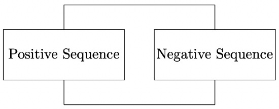Figure 2: Sequence Connections For A Line-To-Line Fault

To illustrate the independence of symmetrical components in balanced networks, consider the transmission line illustrated back in Figure 20 of Installment 3 of these notes. The expressions for voltage drop in the lines may be written as a single vector expression:

\[\ \underline{V}_{p h 1}-\underline{V}_{p h 2}=j \omega \underline{\underline{L}}_{p h} \underline{I}_{p h}\label{27} \]

where

\[\ \underline{V}_{p h}=\left[\begin{array}{l}
\underline{V}_{a} \\
\underline{V}_{b} \\
\underline{V}_{c}
\end{array}\right]\label{28} \]

\[\ \underline{I}_{p h}=\left[\begin{array}{l}
\underline{I}_{a} \\
\underline{I}_{b} \\
\underline{I}_{c}
\end{array}\right]\label{29} \]

\[\ \underline{\underline{L}}_{p h}=\left[\begin{array}{lll}
L & M & M \\
M & L & M \\
M & M & L
\end{array}\right]\label{30} \]

Note that the symmetrical component transformation (4) may be written in compact form:

\[\ \underline{V}_{s}=\underline{\underline{T }V}_{p}\label{31} \]

where

\[\ \underline{\underline{T}}=\frac{1}{3}\left[\begin{array}{lll}
1 & \underline{a} & \underline{a}^{2} \\
1 & \underline{a}^{2} & \underline{a} \\
1 & 1 & 1
\end{array}\right]\label{32} \]

and \(\ \underline{V}_{s}\) is the vector of sequence voltages:

\[\ \underline{V}_{s}=\left[\begin{array}{l}
\underline{V}_{1} \\
\underline{V}_{2} \\
\underline{V}_{0}
\end{array}\right]\label{33} \]

Rewriting (27) using the inverse of (31):

\[\ \underline{\underline{T}}^{-1} \underline{V}_{s 1}-\underline{\underline{T}}^{-1} \underline{V}_{s 2}=j \omega \underline{\underline{L}}_{p h} \underline{\underline{T}}^{-1} \underline{I}_{s}\label{34} \]

Then transforming to get sequence voltages:

\[\ \underline{V}_{s 1}-\underline{V}_{s 2}=j \omega \underline{\underline{T L}}_ {p h} \underline{\underline{T}}^{-1} \underline{I}_{s}\label{35} \]

The sequence inductance matrix is defined by carrying out the operation indicated:

\[\ \underline{\underline{L}}_{s}=\underline{\underline{T L}}_{p h} \underline{\underline{T}}^{-1}\label{36} \]

which is:

\[\ \underline{\underline{L}}_{s}=\left[\begin{array}{ccc}
L-M & 0 & 0 \\
0 & L-M & 0 \\
0 & 0 & L+2 M
\end{array}\right]\label{37} \]

Thus the coupled set of expressions which described the transmission line in phase variables becomes an uncoupled set of expressions in the symmetrical components:

\[\ \underline{V}_{11}-\underline{V}_{12}=j \omega(L-M) \underline{I}_{1}\label{38} \]

\[\ \underline{V}_{21}-\underline{V}_{22}=j \omega(L-M) \underline{I}_{2}\label{39} \]

\[\ \underline{V}_{01}-\underline{V}_{02}=j \omega(L+2 M) \underline{I}_{0}\label{40} \]

The positive, negative and zero sequence impedances of the balanced transmission line are then:

\[\ \underline{Z}_{1}=\underline{Z}_{2}=j \omega(L-M)\label{41} \]

\[\ \underline{Z}_{0} \quad=j \omega(L+2 M)\label{42} \]

So, in analysis of networks with transmission lines, it is now possible to replace the lines with three independent, single- phase networks.

Consider next a balanced three-phase load with its neutral connected to ground through an impedance as shown in Figure 3.

The symmetrical component voltage-current relationship for this network is found simply, by assuming positive, negative and zero sequence currents and finding the corresponding voltages. If this is done, it is found that the symmetrical components are independent, and that the voltagecurrent relationships are:

\[\ \underline{V}_{1}=\underline{Z I}_{1}\label{43} \]

\[\ \underline{V}_{2}=\underline{Z I}_{2}\label{44} \]

\[\ \underline{V}_{0}=\left(\underline{Z}+3 \underline{Z}_{g}\right) \underline{I}_{0}\label{45} \]

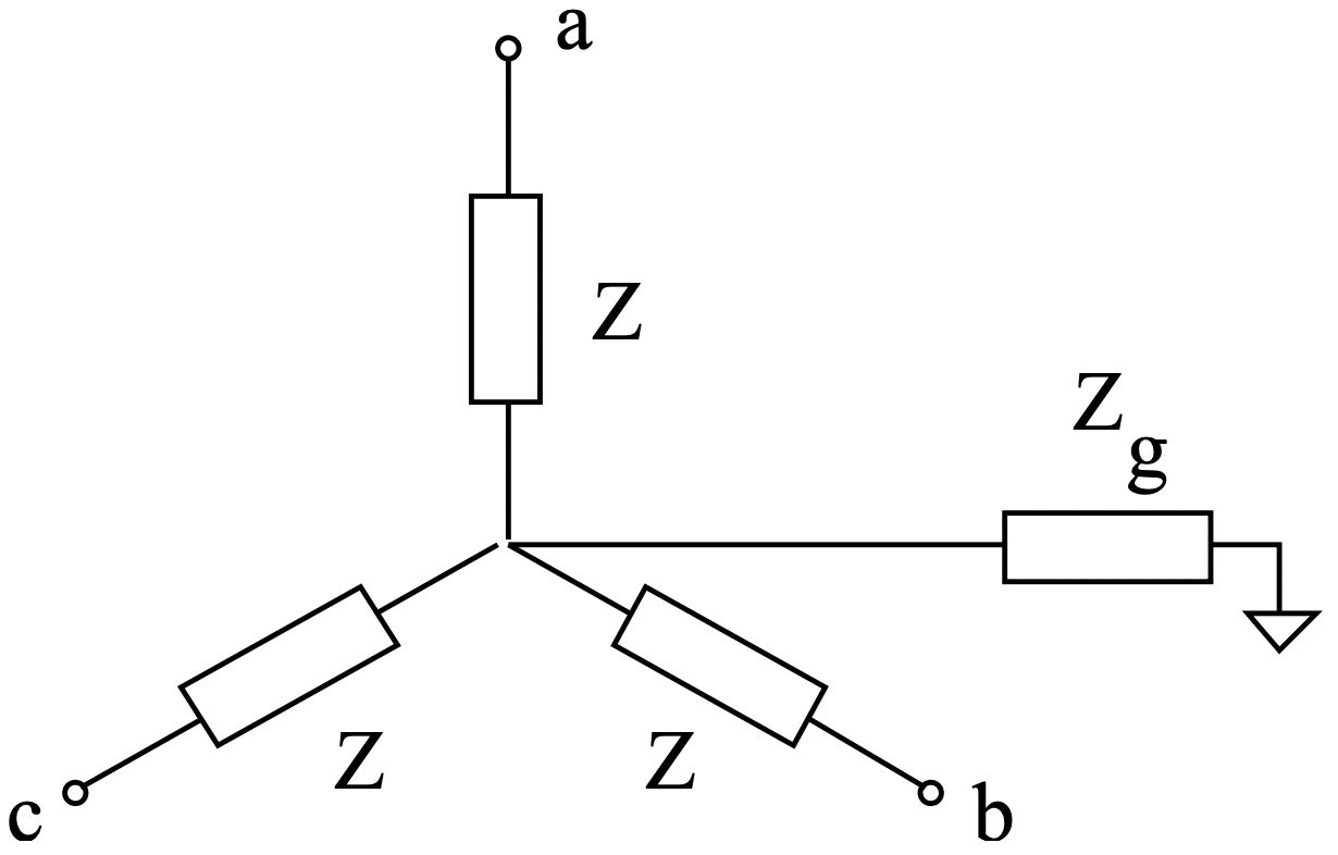Figure 3: Balanced Load With Neutral Impedance