8.1: Energy Conversion Process-

In a motor the energy conversion process can be thought of in simple terms. In “steady state”, electric power input to the machine is just the sum of electric power inputs to the different phase terminals:

\(\ P_{e}=\sum_{i} v_{i} i_{i}\)

Mechanical power is torque times speed:

\(\ P_{m}=T \Omega\)

And the sum of the losses is the difference:

\(\ P_{d}=P_{e}-P_{m}\)

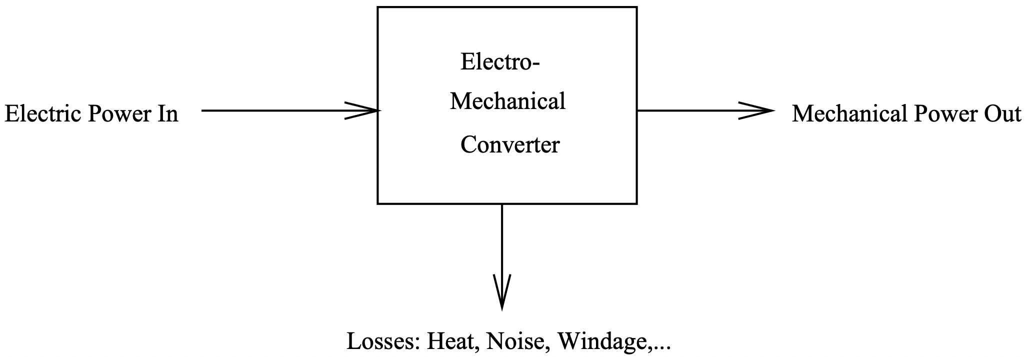Figure 1: Energy Conversion Process

It will sometimes be convenient to employ the fact that, in most machines, dissipation is small enough to approximate mechanical power with electrical power. In fact, there are many situations in which the loss mechanism is known well enough that it can be idealized away. The “thermodynamic” arguments for force density take advantage of this and employ a “conservative” or lossless energy conversion system.

Energy Approach to Electromagnetic Forces:

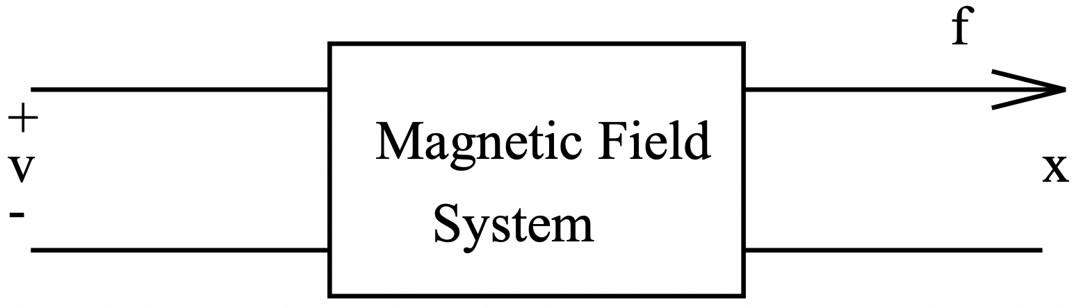Figure 2: Conservative Magnetic Field System

To start, consider some electromechanical system which has two sets of “terminals”, electrical and mechanical, as shown in Figure 2. If the system stores energy in magnetic fields, the energy stored depends on the state of the system, defined by (in this case) two of the identifiable variables: flux \(\ (\lambda)\), current \(\ (i)\) and mechanical position \(\ (x)\). In fact, with only a little reflection, you should be able to convince yourself that this state is a single-valued function of two variables and that the energy stored is independent of how the system was brought to this state.

Now, all electromechanical converters have loss mechanisms and so are not themselves conservative. However, the magnetic field system that produces force is, in principle, conservative in the sense that its state and stored energy can be described by only two variables. The “history” of the system is not important.

It is possible to chose the variables in such a way that electrical power into this conservative system is:

\(\ P^{e}=v i=i \frac{d \lambda}{d t}\)

Similarly, mechanical power out of the system is:

\(\ P^{m}=f^{e} \frac{d x}{d t}\)

The difference between these two is the rate of change of energy stored in the system:

\(\ \frac{d W_{m}}{d t}=P^{e}-P^{m}\)

It is then possible to compute the change in energy required to take the system from one state to another by:

\(\ W_{m}(a)-W_{m}(b)=\int_{b}^{a} i d \lambda-f^{e} d x\)

where the two states of the system are described by \(\ a=\left(\lambda_{a}, x_{a}\right)\) and \(\ b=\left(\lambda_{b}, x_{b}\right)\)

If the energy stored in the system is described by two state variables, \(\ \lambda\) and \(\ x\), the total differential of stored energy is:

\(\ d W_{m}=\frac{\partial W_{m}}{\partial \lambda} d \lambda+\frac{\partial W_{m}}{\partial x} d x\)

and it is also:

\(\ d W_{m}=i d \lambda-f^{e} d x\)

So that we can make a direct equivalence between the derivatives and:

\(\ f^{e}=-\frac{\partial W_{m}}{\partial x}\)

This generalizes in the case of multiple electrical terminals and/or multiple mechanical terminals. For example, a situation with multiple electrical terminals will have:

\(\ d W_{m}=\sum_{k} i_{k} d \lambda_{k}-f^{e} d x\)

And the case of rotary, as opposed to linear, motion has in place of force \(\ f^{e}\) and displacement \(\ x\), torque \(\ T^{e}\) and angular displacement \(\ \theta\).

In many cases we might consider a system which is electricaly linear, in which case inductance is a function only of the mechanical position \(\ x\).

\(\ \lambda(x)=L(x) i\)

In this case, assuming that the energy integral is carried out from \(\ \lambda=0\) (so that the part of the integral carried out over \(\ x\) is zero),

\(\ W_{m}=\int_{0}^{\lambda} \frac{1}{L(x)} \lambda d \lambda=\frac{1}{2} \frac{\lambda^{2}}{L(x)}\)

This makes

\(\ f^{e}=-\frac{1}{2} \lambda^{2} \frac{\partial}{\partial x} \frac{1}{L(x)}\)

Note that this is numerically equivalent to

\(\ f^{e}=-\frac{1}{2} i^{2} \frac{\partial}{\partial x} L(x)\)

This is true only in the case of a linear system. Note that substituting \(\ L(x) i=\lambda\) too early in the derivation produces erroneous results: in the case of a linear system it is a sign error, but in the case of a nonlinear system it is just wrong.

Coenergy

We often will describe systems in terms of inductance rather than its reciprocal, so that current, rather than flux, appears to be the relevant variable. It is convenient to derive a new energy variable, which we will call co-energy, by:

\(\ W_{m}^{\prime}=\sum_{i} \lambda_{i} i_{i}-W_{m}\)

and in this case it is quite easy to show that the energy differential is (for a single mechanical variable) simply:

\(\ d W_{m}^{\prime}=\sum_{k} \lambda_{k} d i_{k}+f^{e} d x\)

so that force produced is:

\(\ f_{e}=\frac{\partial W_{m}^{\prime}}{\partial x}\)

Consider a simple electric machine example in which there is a single winding on a rotor (call it the field winding and a polyphase armature. Suppose the rotor is round so that we can describe the flux linkages as:

\(\ \begin{array}{l}
\lambda_{a}=L_{a} i_{a}+L_{a b} i_{b}+L_{a b} i_{c}+M \cos (p \theta) i_{f} \\
\lambda_{b}=L_{a b} i_{a}+L_{a} i_{b}+L_{a b} i_{c}+M \cos \left(p \theta-\frac{2 \pi}{3}\right) i_{f} \\
\lambda_{c}=L_{a b} i_{a}+L_{a b} i_{b}+L_{a} i_{c}+M \cos \left(p \theta+\frac{2 \pi}{3}\right) i_{f} \\
\lambda_{f}=M \cos (p \theta) i_{a}+M \cos \left(p \theta-\frac{2 \pi}{3}\right) i_{b}+M \cos \left(p \theta+\frac{2 \pi}{3}\right)+L_{f} i_{f}
\end{array}\)

Now, this system can be simply described in terms of coenergy. With multiple excitation it is important to exercise some care in taking the coenergy integral (to ensure that it is taken over a valid path in the multi-dimensional space). In our case there are actually five dimensions, but only four are important since we can position the rotor with all currents at zero so there is no contribution to coenergy from setting rotor position. Suppose the rotor is at some angle \(\ \theta\) and that the four currents have values \(\ i_{a 0}\), \(\ i_{b 0}\), \(\ i_{c 0}\) and \(\ i_{f 0}\). One of many correct path integrals to take would be:

\(\ \begin{array}{l}
W_{m}^{\prime} &=\int_{0}^{i_{a 0}} L_{a} i_{a} d i_{a} \\
&+\int_{0}^{i_{b 0}}\left(L_{a b} i_{a 0}+L_{a} i_{b}\right) d i_{b}\\
&+\int_{0}^{i_{c 0}}\left(L_{a b} i_{a 0}+L_{a b} i_{b 0}+L_{a} i_{c}\right) d i_{c} \\
&+\int_{0}^{i_{f 0}}\left(M \cos (p \theta) i_{a 0}+M \cos \left(p \theta-\frac{2 \pi}{3}\right) i_{b 0}+M \cos \left(p \theta+\frac{2 \pi}{3}\right) i_{c 0}+L_{f} i_{f}\right) d i_{f}
\end{array}\)

The result is:

\(\ \begin{aligned}
W_{m}^{\prime}&= \frac{1}{2} L_{a}\left(i_{a 0}^{2}+i_{b 0}^{2}+i_{c o}^{2}\right)+L_{a b}\left(i_{a o} i_{b 0}+i_{a o} i_{c 0}+i_{c o} i_{b 0}\right) \\
&+M i_{f 0}\left(i_{a 0} \cos (p \theta)+i_{b 0} \cos \left(p \theta-\frac{2 \pi}{3}\right)+i_{c 0} \cos \left(p \theta+\frac{2 \pi}{3}\right)\right)+\frac{1}{2} L_{f} i_{f 0}^{2}
\end{aligned}\)

If there is no variation of the stator inductances with rotor position \(\ \theta\), (which would be the case if the rotor were perfectly round), the terms that involve \(\ L_{a}\) and \(\ \left.L_{(} a b\right)\) contribute zero so that torque is given by:

\(\ T_{e}=\frac{\partial W_{m}^{\prime}}{\partial \theta}=-p M i_{f 0}\left(i_{a 0} \sin (p \theta)+i_{b 0} \sin \left(p \theta-\frac{2 \pi}{3}\right)+i_{c o} \sin \left(p \theta+\frac{2 \pi}{3}\right)\right)\)

We will return to this type of machine in subsequent chapters.

Continuum Energy Flow

At this point, it is instructive to think of electromagnetic energy flow as described by Poynting’s Theorem:

\(\ \vec{S}=\vec{E} \times \vec{H}\)

Energy flow \(\ \vec{S}\), called Poynting’s Vector, describes electromagnetic power in terms of electric and magnetic fields. It is power density: power per unit area, with units in the SI system of units of watts per square meter.

To calculate electromagnetic power into some volume of space, we can integrate Poyting’s Vector over the surface of that volume, and then using the divergence theorem:

\(\ P=-\oiint \vec{S} \cdot \vec{n} d a=-\int_{\mathrm{VOl}} \nabla \cdot \vec{S} d v\)

Now, the divergence of the Poynting Vector is, using a vector identity:

\(\ \begin{aligned}
\nabla \cdot \vec{S} &=\nabla \cdot(\vec{E} \times \vec{H})=\vec{H} \cdot \nabla \times \vec{E}-\vec{E} \cdot \nabla \times \vec{H} \\
&=-\vec{H} \cdot \frac{\partial \vec{B}}{\partial t}-\vec{E} \cdot \vec{J}
\end{aligned}\)

The power crossing into a region of space is then:

\(\ P=\int_{\mathrm{vol}}\left(\vec{E} \cdot \vec{J}+\vec{H} \cdot \frac{\partial \vec{B}}{\partial t}\right) d v\)

Now, in the absence of material motion, interpretation of the two terms in this equation is fairly simple. The first term describes dissipation:

\(\ \vec{E} \cdot \vec{J}=|\vec{E}|^{2} \sigma=|\vec{J}|^{2} \rho\)

The second term is interpreted as rate of change of magnetic stored energy. In the absence of hysteresis it is:

\(\ \frac{\partial W_{m}}{\partial t}=\vec{H} \cdot \frac{\partial \vec{B}}{\partial t}\)

Note that in the case of free space,

\(\ \vec{H} \cdot \frac{\partial \vec{B}}{\partial t}=\mu_{0} \vec{H} \cdot \frac{\partial \vec{H}}{\partial t}=\frac{\partial}{\partial t}\left(\frac{1}{2} \mu_{0}|\vec{H}|^{2}\right)\)

which is straightforwardedly interpreted as rate of change of magnetic stored energy density:

\(\ W_{m}=\frac{1}{2} \mu_{0}|H|^{2}\)

Some materials exhibit hysteretic behavior, in which stored energy is not a single valued function of either \(\ \vec{B}\) or \(\ \vec{H}\), and we will consider that case anon.

Material Motion

In the presence of material motion \(\ \vec{v}\), electric field \(\ \overrightarrow{E^{\prime}}\) in a “moving” frame is related to electric field \(\ \vec{E}\) in a “stationary” frame and to magnetic field \(\ \vec{B}\) by:

\(\ \vec{E}^{\prime}=\vec{E}+\vec{v} \times \vec{B}\)

This is an experimental result obtained by observing charged particles moving in combined electric and magnetic fields. It is a relatavistic expression, so that the qualifiers “moving” and “stationary” are themselves relative. The electric fields are what would be observed in either frame. In MQS systems, the magnetic flux density \(\ \vec{B}\) is the same in both frames.

The term relating to current density becomes:

\(\ \vec{E} \cdot \vec{J}=\left(\vec{E}^{\prime}-\vec{v} \times \vec{B}\right) \cdot \vec{J}\)

We can interpret \(\ \vec{E}^{\prime} \cdot \vec{J}\) as dissipation, but the second term bears a little examination. Note that it is in the form of a vector triple (scalar) product:

\(\ -\vec{v} \times \vec{B} \cdot \vec{J}=-\vec{v} \cdot \vec{B} \times \vec{J}=-\vec{v} \cdot \vec{J} \times \vec{B}\)

This is in the form of velocity times force density and represents power conversion from electromagnetic to mechanical form. This is consistent with the Lorentz force law (also experimentally observed):

\(\ \vec{F}=\vec{J} \times \vec{B}\)

This last expression is yet another way of describing energy conversion processes in electric machinery, as the component of apparent electric field produced by material motion through a magnetic field, when reacted against by a current, produces energy conversion to mechanical form rather than dissipation.

Additional Issues in Energy Methods

There are two more important and interesting issues to consider as we study the development of forces of electromagnetic origin and their calculation using energy methods. These concern situations which are not simply representable by lumped parameters and situations that involve permanent magnets.

Coenergy in Continuous Media

Consider a system with not just a multiplicity of circuits but a continuum of current-carrying paths. In that case we could identify the co-energy as:

\(\ W_{m}^{\prime}=\int_{\text {area }} \int \lambda(\vec{a}) d \vec{J} \cdot d \vec{a}\)

where that area is chosen to cut all of the current carrying conductors. This area can be picked to be perpedicular to each of the current filaments since the divergence of current is zero. The flux \(\ \lambda\) is calculated over a path that coincides with each current filament (such paths exist since current has zero divergence). Then the flux is:

\(\ \lambda(\vec{a})=\int \vec{B} \cdot d \vec{n}\)

Now, if we use the vector potential \(\ \vec{A}\) for which the magnetic flux density is:

\(\ \vec{B}=\nabla \times \vec{A}\)

the flux linked by any one of the current filaments is:

\(\ \lambda(\vec{a})=\oint \vec{A} \cdot d \vec{\ell}\)

Now: it is possible to make \(\ d \vec{\ell}\) coincide with \(\ d \vec{a}\) and be parallel to the current filaments, so that:

\(\ W_{m}^{\prime}=\int_{\mathrm{Vol}} \vec{A} \cdot d \vec{J} d v\)

Permanent Magnets

Permanent magnets are becoming an even more important element in electric machine systems. Often systems with permanent magnets are approached in a relatively ad-hoc way, made equivalent to a current that produces the same MMF as the magnet itself.

The constitutive relationship for a permanent magnet relates the magnetic flux density \(\ \vec{B}\) to magnetic field \(\ \vec{H}\) and the property of the magnet itself, the magnetization \(\ \vec{M}\).

\(\ \vec{B}=\mu_{0}(\vec{H}+\vec{M})\)

Now, the effect of the magnetization is to act as if there were a current (called an amperian current) with density:

\(\ \vec{J}^{*}=\nabla \times \vec{M}\)

Note that this amperian current “acts” just like ordinary current in making magnetic flux density. Magnetic co-energy is:

\(\ W_{m}^{\prime}=\int_{\mathrm{vol}} \vec{A} \cdot \nabla \times d \vec{M} d v\)

Next, note the vector identity

\(\ \nabla \cdot(\vec{C} \times \vec{D})=\vec{D} \cdot(\nabla \times \vec{C})-\vec{C} \cdot(\nabla \times \vec{D})\)

So that:

\(\ W_{m}^{\prime}=\int_{\mathrm{vol}}-\nabla \cdot(\vec{A} \times d \vec{M}) d v+\int_{\mathrm{vol}}(\nabla \times \vec{A}) \cdot d \vec{M} d v\)

Then, noting that \(\ \vec{B}=\nabla \times \vec{A}\):

\(\ W_{m}^{\prime}=-\oiint \vec{A} \times d \vec{M} d \vec{s}+\int_{\mathrm{vol}} \vec{B} \cdot d \vec{M} d v\)

The first of these integrals (closed surface) vanishes if it is taken over a surface just outside the magnet, where \(\ \vec{M}\) is zero. Thus the magnetic co-energy in a system with only a permanent magnet source is

\(\ W_{m}^{\prime}=\int_{\mathrm{VOl}} \vec{B} \cdot d \vec{M} d v\)

Adding current carrying coils to such a system is done in the obvious way.

Electric Machine Description:

Actually, this description shows a conventional induction motor. This is a very common type of electric machine and will serve as a reference point. Most other electric machines operate in a fashion which is the same as the induction machine or which differ in ways which are easy to reference to the induction machine.

Consider the simplified machine drawing shown in Figure 3. Most (but not all!) machines we will be studying have essentially this morphology. The rotor of the machine is mounted on a shaft which is supported on some sort of bearing(s). Usually, but not always, the rotor is inside. I have drawn a rotor which is round, but this does not need to be the case. I have also indicated rotor conductors, but sometimes the rotor has permanent magnets either fastened to it or inside, and sometimes (as in Variable Reluctance Machines) it is just an oddly shaped piece of steel. The stator is, in this drawing, on the outside and has windings. With most of the machines we will be dealing with, the stator winding is the armature, or electrical power input element. (In DC and Universal motors this is reversed, with the armature contained on the rotor: we will deal with these later).

In most electrical machines the rotor and the stator are made of highly magnetically permeable materials: steel or magnetic iron. In many common machines such as induction motors the rotor and stator are both made up of thin sheets of silicon steel. Punched into those sheets are slots which contain the rotor and stator conductors.

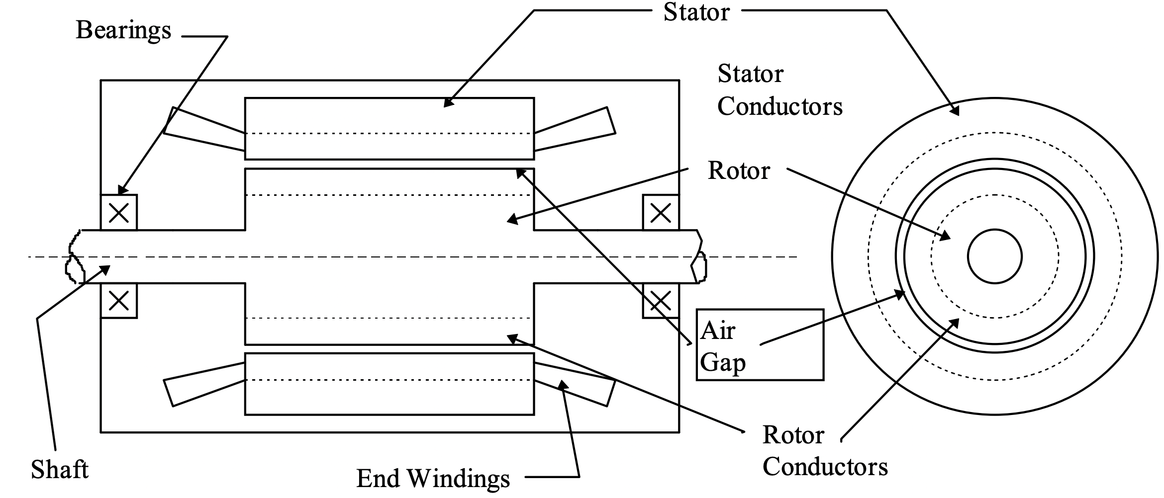Figure 3: Form of Electric Machine

Figure 4 is a picture of part of an induction machine distorted so that the air-gap is straightened out (as if the machine had infinite radius). This is actually a convenient way of drawing the machine and, we will find, leads to useful methods of analysis.

What is important to note for now is that the machine has an air gap g which is relatively small (that is, the gap dimension is much less than the machine radius r). The machine also has a physical length l. The electric machine works by producing a shear stress in the air-gap (with of course side effects such as production of “back voltage”). It is possible to define the average airgap shear stress, which we will refer to as \(\ \tau\). Total developed torque is force over the surface area times moment (which is rotor radius):

\(\ T=2 \pi r^{2} \ell<\tau>\)

Power transferred by this device is just torque times speed, which is the same as force times surface velocity, since surface velocity is \(\ u=r \Omega\):

\(\ P_{m}=\Omega T=2 \pi r \ell<\tau>u\)

If we note that active rotor volume is \(\ \pi r^{2} \ell\), the ratio of torque to volume is just:

\(\ \frac{T}{V_{r}}=2<\tau>\)

Now, determining what can be done in a volume of machine involves two things. First, it is clear that the volume we have calculated here is not the whole machine volume, since it does not include the stator. The actual estimate of total machine volume from the rotor volume is actually quite complex and detailed and we will leave that one for later. Second, we need to estimate the value of the useful average shear stress. Suppose both the radial flux density Br and the stator surface current density Kz are sinusoidal flux waves of the form:

\(\ B_{r}=\sqrt{2} B_{0} \cos (p \theta-\omega t)\)

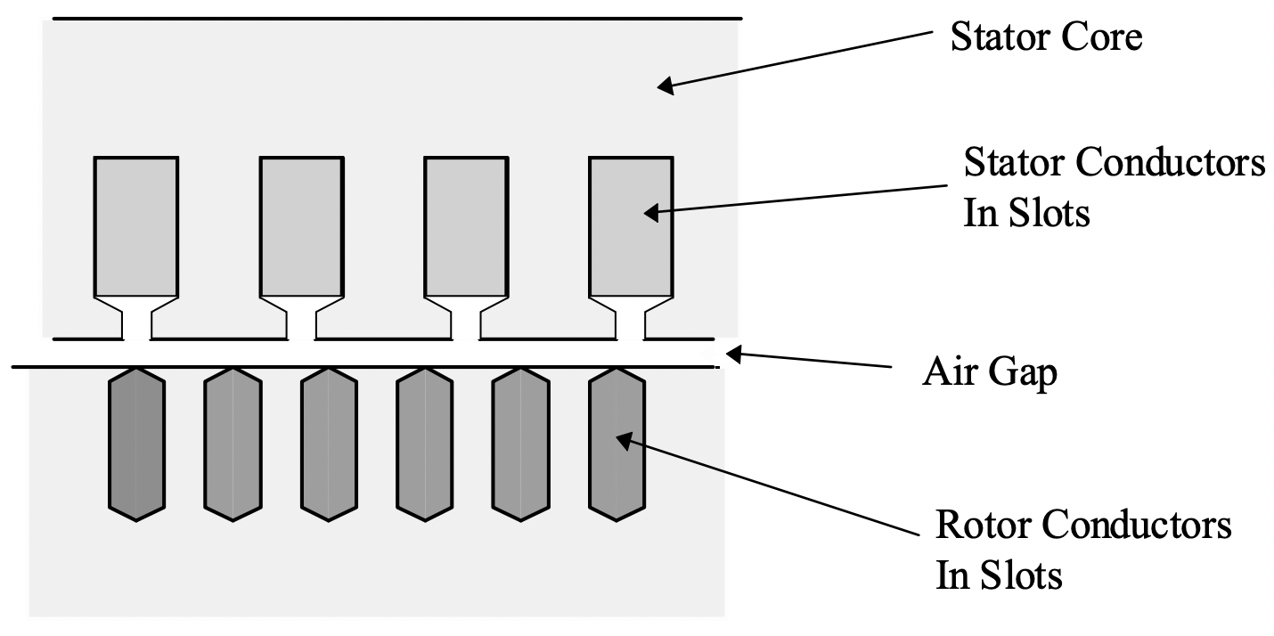Figure 4: Windings in Slots

\(\ K_{z}=\sqrt{2} K_{0} \cos (p \theta-\omega t)\)

Note that this assumes these two quantities are exactly in phase, or oriented to ideally produce torque, so we are going to get an “optimistic” bound here. Then the average value of surface traction is:

\(\ <\tau>=\frac{1}{2 \pi} \int_{0}^{2 \pi} B_{r} K_{z} d \theta=B_{0} K_{0}\)

This actually makes some sense in view of the empirically derived Lorentz Force Law: Given a (vector) current density and a (vector) flux density. In the absence of magnetic materials (those with permeability different from that of free space), the observed force on a conductor is:

\(\ \vec{F}=\vec{J} \times \vec{B}\)

Where \(\ \vec{J}\) is the vector describing current density \(\ \left(A / m^{2}\right)\) and \(\ \vec{B}\) is the magnetic flux density (T). This is actually enough to describe the forces we see in many machines, but since electric machines have permeable magnetic material and since magnetic fields produce forces on permeable material even in the absence of macroscopic currents it is necessary to observe how force appears on such material. A suitable empirical expression for force density is:

\(\ \vec{F}=\vec{J} \times \vec{B}-\frac{1}{2}(\vec{H} \cdot \vec{H}) \nabla \mu\)

where \(\ \vec{H}\) is the magnetic field intensity and \(\ \mu\) is the permeability.

Now, note that current density is the curl of magnetic field intensity, so that:

\(\ \begin{aligned}
\vec{F} &=(\nabla \times \vec{H}) \times \mu \vec{H}-\frac{1}{2}(\vec{H} \cdot \vec{H}) \nabla \mu \\
&=\mu(\nabla \times \vec{H}) \times \vec{H}-\frac{1}{2}(\vec{H} \cdot \vec{H}) \nabla \mu
\end{aligned}\)

And, since:

\(\ (\nabla \times \vec{H}) \times \vec{H}=(\vec{H} \cdot \nabla) \vec{H}-\frac{1}{2} \nabla(\vec{H} \cdot \vec{H})\)

force density is:

\(\ \begin{aligned}
\vec{F} &=\mu(\vec{H} \cdot \nabla) \vec{H}-\frac{1}{2} \mu \nabla(\vec{H} \cdot \vec{H})-\frac{1}{2}(\vec{H} \cdot \vec{H}) \nabla \mu \\
&=\mu(\vec{H} \cdot \nabla) \vec{H}-\nabla\left(\frac{1}{2} \mu(\vec{H} \cdot \vec{H})\right)
\end{aligned}\)

This expression can be written by components: the component of force in the i’th dimension is:

\(\ F_{i}=\mu \sum_{k}\left(H_{k} \frac{\partial}{\partial x_{k}}\right) H_{i}-\frac{\partial}{\partial x_{i}}\left(\frac{1}{2} \mu \sum_{k} H_{k}^{2}\right)\)

Now, see that we can write the divergence of magnetic flux density as:

\(\ \nabla \cdot \vec{B}=\sum_{k} \frac{\partial}{\partial x_{k}} \mu H_{k}=0\)

and

\(\ \mu \sum_{k}\left(H_{k} \frac{\partial}{\partial x_{k}}\right) H_{i}=\sum_{k} \frac{\partial}{\partial x_{k}} \mu H_{k} H_{i}-H_{i} \sum_{k} \frac{\partial}{\partial x_{k}} \mu H_{k}\)

but since the last term in that is zero, we can write force density as:

\(\ F_{k}=\frac{\partial}{\partial x_{i}}\left(\mu H_{i} H_{k}-\frac{\mu}{2} \delta_{i k} \sum_{n} H_{n}^{2}\right)\)

where we have used the Kroneker delta \(\ \delta_{i k}=1\) if \(\ i=k\), 0 otherwise.

Note that this force density is in the form of the divergence of a tensor:

\(\ F_{k}=\frac{\partial}{\partial x_{i}} T_{i k}\)

or

\(\ \vec{F}=\nabla \cdot \underline{\underline{T}}\)

In this case, force on some object that can be surrounded by a closed surface can be found by using the divergence theorem:

\(\ \vec{f}=\int_{\mathrm{vol}} \vec{F} d v=\int_{\mathrm{vol}} \nabla \cdot \underline{\underline{T}} d v=\oiint \underline{\underline{T}} \cdot \vec{n} d a\)

or, if we note surface traction to be \(\ \tau_{i}=\sum_{k} T_{i k} n_{k}\), where n is the surface normal vector, then the total force in direction i is just:

\(\ \vec{f}=\oint_{s} \tau_{i} d a=\oint \sum_{k} T_{i k} n_{k} d a\)

The interpretation of all of this is less difficult than the notation suggests. This field description of forces gives us a simple picture of surface traction, the force per unit area on a surface. If we just integrate this traction over the area of some body we get the whole force on the body. Note that this works if we integrate the traction over a surface that is itself in free space but which surrounds the body (because we can impose no force on free space).

Note one more thing about this notation. Sometimes when subscripts are repeated as they are here the summation symbol is omitted. Thus we would write \(\ \tau_{i}=\sum_{k} T_{i k} n_{k}=T_{i k} n_{k}\).

Now, if we go back to the case of a circular cylinder and are interested in torque, it is pretty clear that we can compute the circumferential force by noting that the normal vector to the cylinder is just the radial unit vector, and then the circumferential traction must simply be:

\(\ \tau_{\theta}=\mu_{0} H_{r} H_{\theta}\)

Simply integrating this over the surface gives azimuthal force, and then multiplying by radius (moment arm) gives torque. The last step is to note that, if the rotor is made of highly permeable material, the azimuthal magnetic field is equal to surface current density.