8.2: Tying the MST and Poynting Approaches Together

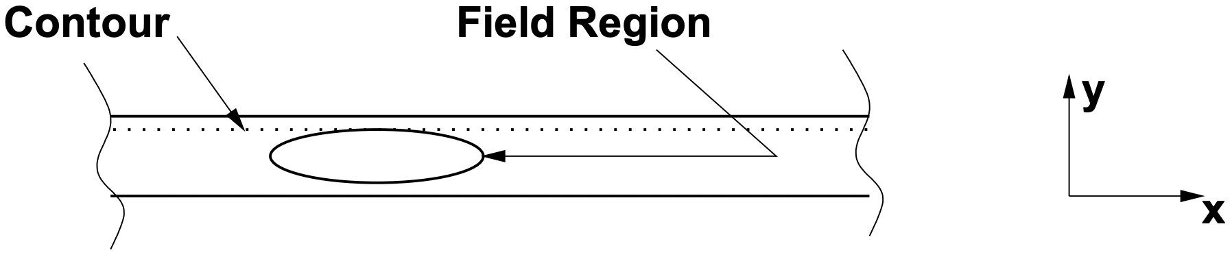Figure 5: Illustrative Region of Space

Now that the stage is set, consider energy flow and force transfer in a narrow region of space as illustrated by Figure 5. The upper and lower surfaces may support currents. Assume that all of the fields, electric and magnetic, are of the form of a traveling wave in the x- direction: \(\ \operatorname{Re}\left\{e^{j(\omega t-k x)}\right\}\).

If we assume that form for the fields and also assume that there is no variation in the z- direction (equivalently, the problem is infinitely long in the z- direction), there can be no x- directed currents because the divergence of current is zero: \(\ \nabla \cdot \vec{J}=0\). In a magnetostatic system this is true of electric field \(\ \vec{E}\) too. Thus we will assume that current is confined to the z- direction and to the two surfaces illustrated in Figure 5, and thus the only important fields are:

\(\ \begin{aligned}
\vec{E} &=\vec{i}_{z} \operatorname{Re}\left\{\underline{E}_{z} e^{j(\omega t-k x)}\right\} \\
\vec{H} &=\vec{i}_{x} \operatorname{Re}\left\{\underline{H}_{x} e^{j(\omega t-k x)}\right\} \\
&+\vec{i}_{y} \operatorname{Re}\left\{\underline{H}_{y} e^{j(\omega t-k x)}\right\}
\end{aligned}\)

We may use Faraday’s Law \(\ \left(\nabla \times \vec{E}=-\frac{\partial \vec{B}}{\partial t}\right)\) to establish the relationship between the electric ∂t and magnetic field: the y- component of Faraday’s Law is:

\(\ j k \underline{E}_{z}=-j \omega \mu_{0} \underline{H}_{y}\)

or

\(\ \underline{E}_{z}=-\frac{\omega}{k} \mu_{0} \underline{H}_{y}\)

The phase velocity \(\ u_{p h}=\frac{\omega}{k}\) is a most important quantity. Note that, if one of the surfaces is moving (as it would be in, say, an induction machine), the frequency and hence the apparent phase velocity, will be shifted by the motion. We will use this fact shortly.

Energy flow through the surface denoted by the dotted line in Figure 5 is the component of Poynting’s Vector in the negative y- direction. The relevant component is:

\(\ S_{y}=(\vec{E} \times \vec{H})_{y}=E_{z} H_{x}=-\frac{\omega}{k} \mu_{0} H_{y} H_{x}\)

Note that this expression contains the xy component of the Maxwell Stress Tensor \(\ T_{x y}=\mu_0H_xH_y\) so that power flow downward through the surface is:

\(\ \mathbf{S}=-S_{y}=\frac{\omega}{k} \mu_{0} H_{x} H_{y}=u_{p h} T_{x y}\)

The average power flow is the same, in this case, for time and for space, and is:

\(\ <\mathbf{S}>=\frac{1}{2} \operatorname{Re}\left\{\underline{E}_{z} \underline{H}_{x}^{*}\right\}=u_{p h} \frac{\mu_{0}}{2} \operatorname{Re}\left\{\underline{H}_{y} \underline{H}_{x}^{*}\right\}\)

We may choose to define a surface impedance:

\(\ \underline{Z}_{s}=\frac{\underline{E}_{z}}{-\underline{H}_{x}}\)

which becomes:

\(\ \underline{Z}_{s}=-\mu_{0} u_{p h} \frac{\underline{H}_{y}}{\underline{H}_{x}}=-\mu_{0} u_{p h} \underline{R}\)

where now we have defined the parameter \(\ \underline{R}\) to be the ratio between y- and x- directed complex field amplitudes. Energy flow through that surface is now:

\(\ \mathbf{S}=-\frac{1}{s} \operatorname{Re}\left\{\underline{E}_{z} \underline{H}_{x}^{*}\right\}=\frac{1}{2} \operatorname{Re}\left\{\left|\underline{H}_{x}\right|^{2} \underline{Z}_{s}\right\}\)