8.3: Simple Description of a Linear Induction Motor

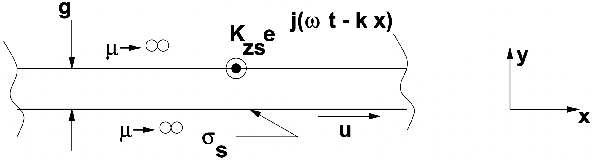Figure 6: Simple Description of Linear Induction Motor

The stage is now set for an almost trivial description of a linear induction motor. Consider the geometry described in Figure 6. Shown here is only the relative motion gap region. This is bounded by two regions of highly permeable material (e.g. iron), comprising the stator and shuttle. On the surface of the stator (the upper region) is a surface current:

\(\ \vec{K}_{s}=\vec{i}_{z} \operatorname{Re}\left\{\underline{K}_{z s} e^{j(\omega t-k x)}\right\}\)

The shuttle is, in this case, moving in the positive x- direction at some velocity \(\ u\). It may also be described as an infinitely permeable region with the capability of supporting a surface current with surface conductivity \(\ \sigma_{s}\), so that \(\ K_{z r}=\sigma_{s} E_{z}\).

Note that Ampere’s Law gives us a boundary condition on magnetic field just below the upper surface of this problem: \(\ H_{x}=K_{z s}\), so that, if we can establish the ratio between y- and x- directed fields at that location,

\(\ <T_{x y}>=\frac{\mu_{0}}{2} \operatorname{Re}\left\{\underline{H}_{y} \underline{H}_{x}^{*}\right\}=\frac{\mu_{0}}{2}\left|\underline{K}_{z s}\right|^{2} \operatorname{Re}\{\underline{R}\}\)

Note that the ratio of fields \(\ \underline{H}_{y} / \underline{H}_{x}=\underline{R}\) is independent of reference frame (it doesn’t matter if we are looking at the fields from the shuttle or the stator), so that the shear stress described by \(\ T_{x y}\) is also frame independent. Now, if the shuttle (lower surface) is moving relative to the upper surface, the velocity of the traveling wave relative to the shuttle is:

\(\ u_{s}=u_{p h}-u=s \frac{\omega}{k}\)

where we have now defined the dimensionless slip s to be the ratio between frequency seen by the shuttle to frequency seen by the stator. We may use this to describe energy flow as described by Poynting’s Theorem. Energy flow in the stator frame is:

\(\ \mathbf{S}_{\text {upper }}=u_{p h} T_{x y}\)

In the frame of the shuttle, however, it is

\(\ \mathbf{S}_{\text {lower }}=u_{s} T_{x y}=s \mathbf{S}_{\text {upper }}\)

Now, the interpretation of this is that energy flow out of the upper surface \(\ \left(\mathbf{S}_{\text {upper }}\right)\) consists of energy converted (mechanical power) plus energy dissipated in the shuttle (which is \(\ \mathbf{S}_{\text {lower }}\) here. The difference between these two power flows, calculated using Poynting’s Theorem, is power converted from electrical to mechanical form:

\(\ \mathbf{S}_{\text {converted }}=\mathbf{S}_{\text {upper }}(1-s)\)

Now, to finish the problem, note that surface current in the shuttle is:

\(\ \underline{K}_{z r}=\underline{E}_{z}^{\prime} \sigma_{s}=-u_{s} \mu_{0} \sigma_{s} \underline{H}_{y}\)

where the electric field \(\ \underline{E^{\prime}}_{z}\) is measured in the frame of the shuttle.

We assume here that the magnetic gap \(\ g\) is small enough that we may assume \(\ k g \ll 1\). Ampere’s Law, taken around a contour that crosses the air-gap and has a normal in the z- direction, yields:

\(\ g \frac{\partial H_{x}}{\partial x}=K_{z s}+K_{z r}\)

In complex amplitudes, this is:

\(\ -j k g \underline{H}_{y}=\underline{K}_{z s}+\underline{K}_{z r}=\underline{K}_{z s}-\mu_{0} u_{s} \sigma_{s} \underline{H}_{y}\)

or, solving for \(\ H_{y}\).

\(\ \underline{H}_{y}=\frac{j K_{z s}}{k g} \frac{1}{1+j \mu_{0} \frac{u_{s} \sigma_{s}}{k g}}\)

Average shear stress is

\(\ \left.<T_{x y}\right\rangle=\frac{\mu_{0}}{2} \operatorname{Re}\left\{\underline{H}_{y} \underline{H}_{x}\right\}=\frac{\mu_{0}}{2} \frac{\left|\underline{K}_{z s}\right|^{2}}{k g} \operatorname{Re}\left\{\frac{j}{1+j \frac{\mu_{0} u_{s} \sigma_{s}}{k g}}\right\}=\frac{\mu_{0}}{2} \frac{\left|\underline{K}_{z s}\right|^{2}}{k g} \frac{\frac{\mu_{0} u_{s} \sigma_{s}}{k g}}{1+\left(\frac{\mu_{0} u_{s} \sigma_{s}}{k g}\right)^{2}}\)