8.4: Surface Impedance of Uniform Conductors

The objective of this section is to describe the calculation of the surface impedance presented by a layer of conductive material. Two problems are considered here. The first considers a layer of linear material backed up by an infinitely permeable surface. This is approximately the situation presented by, for example, surface mounted permanent magnets and is probably a decent approximation to the conduction mechanism that would be responsible for loss due to asynchronous harmonics in these machines. It is also appropriate for use in estimating losses in solid rotor induction machines and in the poles of turbogenerators. The second problem, which we do not work here but simply present the previously worked solution, concerns saturating ferromagnetic material.

Linear Case

The situation and coordinate system are shown in Figure 7. The conductive layer is of thicknes \(\ T\) and has conductivity \(\ \sigma\) and permeability \(\ \mu_{0}\). To keep the mathematical expressions within bounds, we assume rectilinear geometry. This assumption will present errors which are small to the extent that curvature of the problem is small compared with the wavenumbers encountered. We presume that the situation is excited, as it would be in an electric machine, by a current sheet of the form \(\ K_{z}=\operatorname{Re}\left\{\underline{K} e^{j(\omega t-k x)}\right\}\).

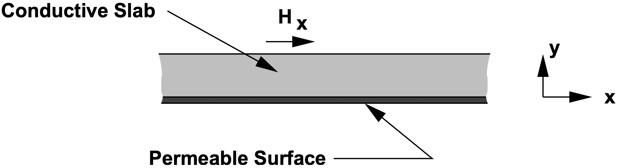Figure 7: Axial View of Magnetic Field Problem

In the conducting material, we must satisfy the diffusion equation:

\(\ \nabla^{2} \bar{H}=\mu_{0} \sigma \frac{\partial \bar{H}}{\partial t}\)

In view of the boundary condition at the back surface of the material, taking that point to be \(\ y=0\), a general solution for the magnetic field in the material is:

\(\ \begin{aligned}
H_{x} &=\operatorname{Re}\left\{A \sinh \alpha y e^{j(\omega t-k x)}\right\} \\
H_{y} &=\operatorname{Re}\left\{j \frac{k}{\alpha} A \cosh \alpha y e^{j(\omega t-k x)}\right\}
\end{aligned}\)

where the coefficient α satisfies:

\(\ \alpha^{2}=j \omega \mu_{0} \sigma+k^{2}\)

and note that the coefficients above are chosen so that \(\ \bar{H}\) has no divergence.

Note that if \(\ k\) is small (that is, if the wavelength of the excitation is large), this spatial coefficient \(\ \alpha\) becomes

\(\ \alpha=\frac{1+j}{\delta}\)

where the skin depth is:

\(\ \delta=\sqrt{\frac{2}{\omega \mu_{0} \sigma}}\)

To obtain surface impedance, we use Faraday’s law:

\(\ \nabla \times \bar{E}=-\frac{\partial \bar{B}}{\partial t}\)

which gives:

\(\ \underline{E}_{z}=-\mu_{0} \frac{\omega}{k} \underline{H}_{y}\)

Now: the “surface current” is just

\(\ \underline{K}_{s}=-\underline{H}_{x}\)

so that the equivalent surface impedance is:

\(\ \underline{Z}=\frac{\underline{E}_{z}}{-\underline{H}_{x}}=j \mu_{0} \frac{\omega}{\alpha} \operatorname{coth} \alpha T\)

A pair of limits are interesting here. Assuming that the wavelength is long so that \(\ k\) is negligible, then if \(\ \alpha T\) is small (i.e. thin material),

\(\ \underline{Z} \rightarrow j \mu_{0} \frac{\omega}{\alpha^{2} T}=\frac{1}{\sigma T}\)

On the other hand as \(\ \alpha T \rightarrow \infty\),

\(\ \underline{Z} \rightarrow \frac{1+j}{\sigma \delta}\)

Next it is necessary to transfer this surface impedance across the air-gap of a machine. So, with reference to Figure 8, assume a new coordinate system in which the surface of impedance \(\ \underline{Z}_{s}\) is located at \(\ y=0\), and we wish to determine the impedance \(\ \underline{Z}=-\underline{E}_{z} / \underline{H}_{x}\) at \(\ y=g\).

In the gap there is no current, so magnetic field can be expressed as the gradient of a scalar potential which obeys Laplace’s equation:

\(\ \bar{H}=-\nabla \psi\)

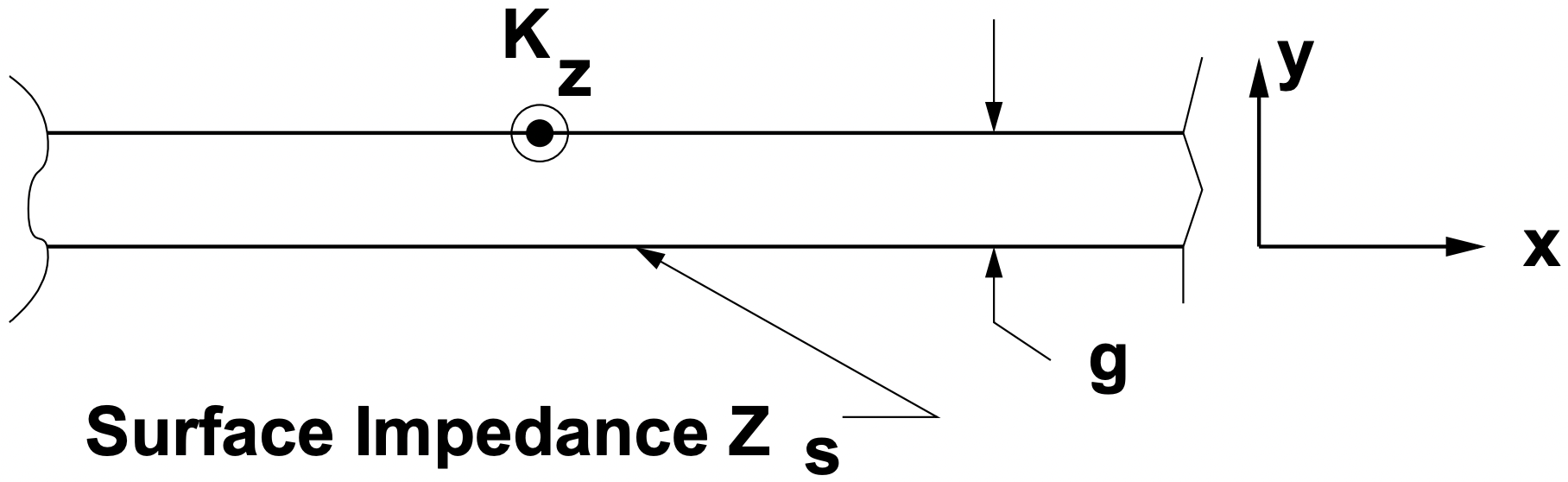Figure 8: Impedance across the air-gap

and

\(\ \nabla^{2} \psi=0\)

Ignoring a common factor of \(\ e^{j(\omega t-k x)}\), we can express \(\ \bar{H}\) in the gap as:

\(\ \begin{array}{l}
\underline{H}_{x}=j k\left(\underline{\psi}_{+} e^{k y}+\underline{\psi}_{-} e^{-k y}\right) \\
\underline{H}_{y}=-k\left(\underline{\psi}_{+} e^{k y}-\underline{\psi}_{-} e^{-k y}\right)
\end{array}\)

At the surface of the rotor,

\(\ \underline{E}_{z}=-\underline{H}_{x} \underline{Z}_{s}\)

or

\(\ -\omega \mu_{0}\left(\underline{\psi}_{+}-\underline{\psi}_{-}\right)=j k \underline{Z}_{s}\left(\underline{\psi}_{+}+\underline{\psi}_{-}\right)\)

and then, at the surface of the stator,

\(\ \underline{Z}=-\frac{\underline{E}_{z}}{\underline{H}_{x}}=j \mu_{0} \frac{\omega}{k} \frac{\underline{\psi}_{+} e^{k g}-\underline{\psi}_{-} e^{-k g}}{\underline{\psi}_{+} e^{k g}+\underline{\psi}_{-} e^{-k g}}\)

A bit of manipulation is required to obtain:

\(\ \underline{Z}=j \mu_{0} \frac{\omega}{k}\left\{\frac{e^{k g}\left(\omega \mu_{0}-j k \underline{Z}_{s}\right)-e^{-k g}\left(\omega \mu_{0}+j k \underline{Z}_{s}\right)}{e^{k g}\left(\omega \mu_{0}-j k \underline{Z}_{s}\right)+e^{-k g}\left(\omega \mu_{0}+j k \underline{Z}_{s}\right)}\right\}\)

It is useful to note that, in the limit of \(\ \underline{Z}_{s} \rightarrow \infty\), this expression approaches the gap impedance

\(\ \underline{Z}_{g}=j \frac{\omega \mu_{0}}{k^{2} g}\)

and, if the gap is small enough that \(\ k g \rightarrow 0\),

\(\ \underline{Z} \rightarrow \underline{Z}_{g} \| \underline{Z}_{s}\)