8.5: Iron

Electric machines employ ferromagnetic materials to carry magnetic flux from and to appropriate places within the machine. Such materials have properties which are interesting, useful and problematical, and the designers of electric machines must deal with this stuff. The purpose of this note is to introduce the most salient properties of the kinds of magnetic materials used in electric machines.

We will be concerned here with materials which exhibit magnetization: flux density is something other than \(\ \vec{B}=\mu_{0} \vec{H}\). Generally, we will speak of hard and soft magnetic materials. Hard materials are those in which the magnetization tends to be permanent, while soft materials are used in magnetic circuits of electric machines and transformers. Since they are related we will find ourselves talking about them either at the same time or in close proximity, even though their uses are widely disparite.

Magnetization:

It is possible to relate, in all materials, magnetic flux density to magnetic field intensity with a consitutive relationship of the form:

\(\ \vec{B}=\mu_{0}(\vec{H}+\vec{M})\)

where magnetic field intensity H and magnetization M are the two important properties. Now, in linear magnetic material magnetization is a simple linear function of magnetic field:

\(\ \vec{M}=\chi_{m} \vec{H}\)

so that the flux density is also a linear function:

\(\ \vec{B}=\mu_{0}\left(1+\chi_{m}\right) \vec{H}\)

Note that in the most general case the magnetic susceptibility cm might be a tensor, leading to flux density being non-colinear with magnetic field intensity. But such a relationship would still be linear. Generally this sort of complexity does not have a major effect on electric machines.

Saturation and Hysteresis

In useful magnetic materials this nice relationship is not correct and we need to take a more general view. We will not deal with the microscopic picture here, except to note that the magnetization is due to the alignment of groups of magnetic dipoles, the groups often called domaines. There are only so many magnetic dipoles available in any given material, so that once the flux density is high enough the material is said to saturate, and the relationship between magnetic flux density and magnetic field intensity is nonlinear.

Shown in Figure 9, for example, is a “saturation curve” for a magnetic sheet steel that is sometimes used in electric machinery. Note the magnetic field intensity is on a logarithmic scale. If this were plotted on linear coordinates the saturation would appear to be quite abrupt.

At this point it is appropriate to note that the units used in magnetic field analysis are not always the same nor even consistent. In almost all systems the unit of flux is the weber (W), which

Courtesy of United States Steel Corporation. (U.S. Steel). U.S. Steel accepts no liability for reliance on any information contained in the graphs shown above.

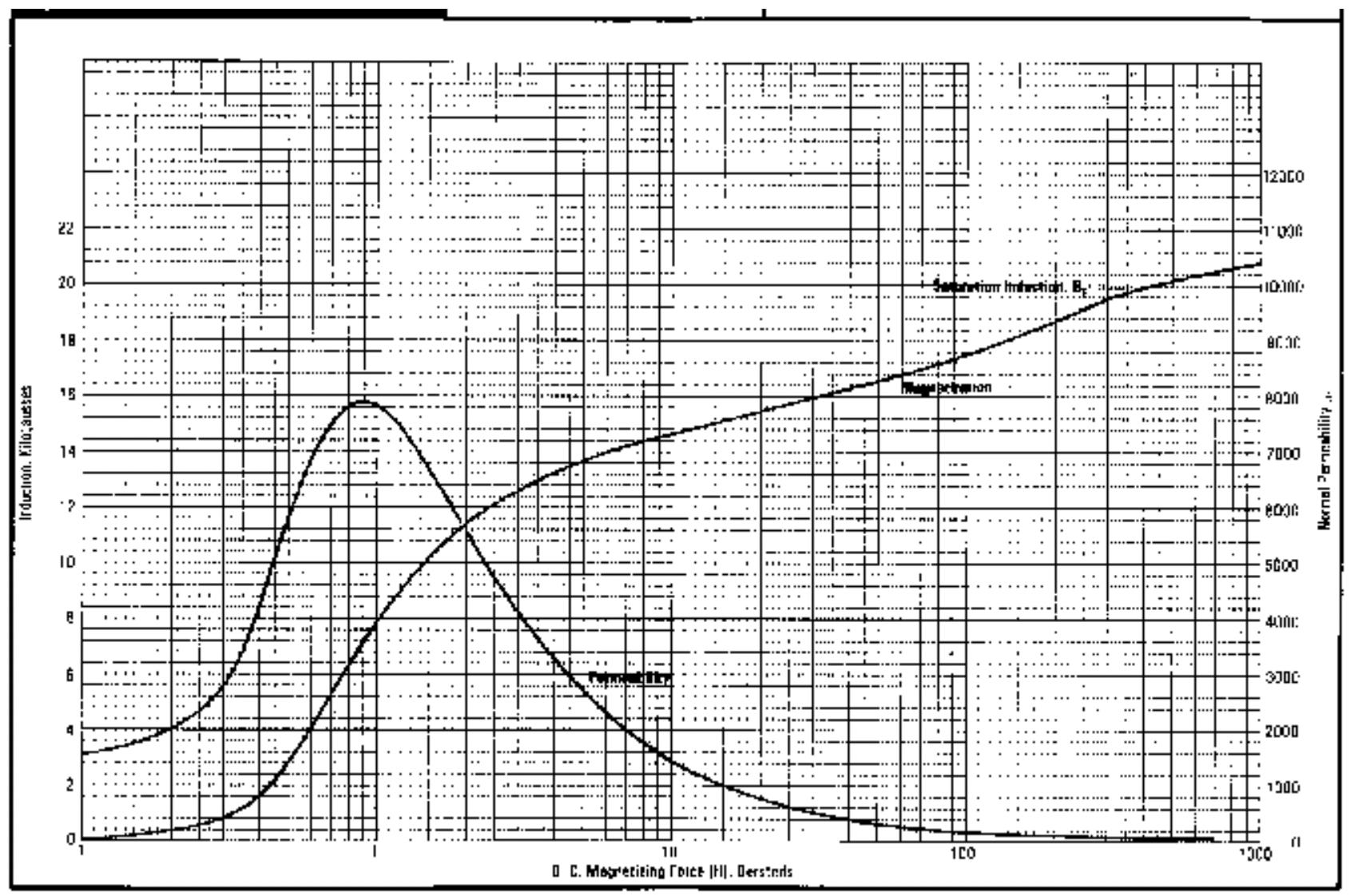
is the same as a volt-second. In SI the unit of flux density is the tesla (T), but many people refer to the gauss (G), which has its origin in CGS. 10,000 G = 1 T. Now it gets worse, because there is an English system measure of flux density generally called kilo-lines per square inch. This is because in the English system the unit of flux is the line. 10⁸ lines is equal to a weber. Thus a Tesla is 64.5 kilolines per square inch.

The SI and CGS units of flux density are easy to reconcile, but the units of magnetic field are a bit harder. In SI we generally measure H in amperes/meter (or ampere-turns per meter). Often, however, you will see magnetic field represented as Oersteds (Oe). One Oe is the same as the magnetic field required to produce one gauss in free space. So 79.577 A/m is one Oe.

In most useful magnetic materials the magnetic domaines tend to be somewhat “sticky”, and a more-than-incremental magnetic field is required to get them to move. This leads to the property called “hysteresis”, both useful and problematical in many magnetic systems.

Hysteresis loops take many forms; a generalized picture of one is shown in Figure 10. Salient features of the hysteresis curve are the remanent magnetization \(\ B_{r}\) and the coercive field \(\ H_{c}\). Note that the actual loop that will be traced out is a function of field amplitude and history. Thus there are many other “minor loops” that might be traced out by the B-H characteristic of a piece of material, depending on just what the fields and fluxes have done and are doing.

Now, hysteresis is important for two reasons. First, it represents the mechanism for “trapping” magnetic flux in a piece of material to form a permanent magnet. We will have more to say about that anon. Second, hysteresis is a loss mechanism. To show this, consider some arbitrary chunk of

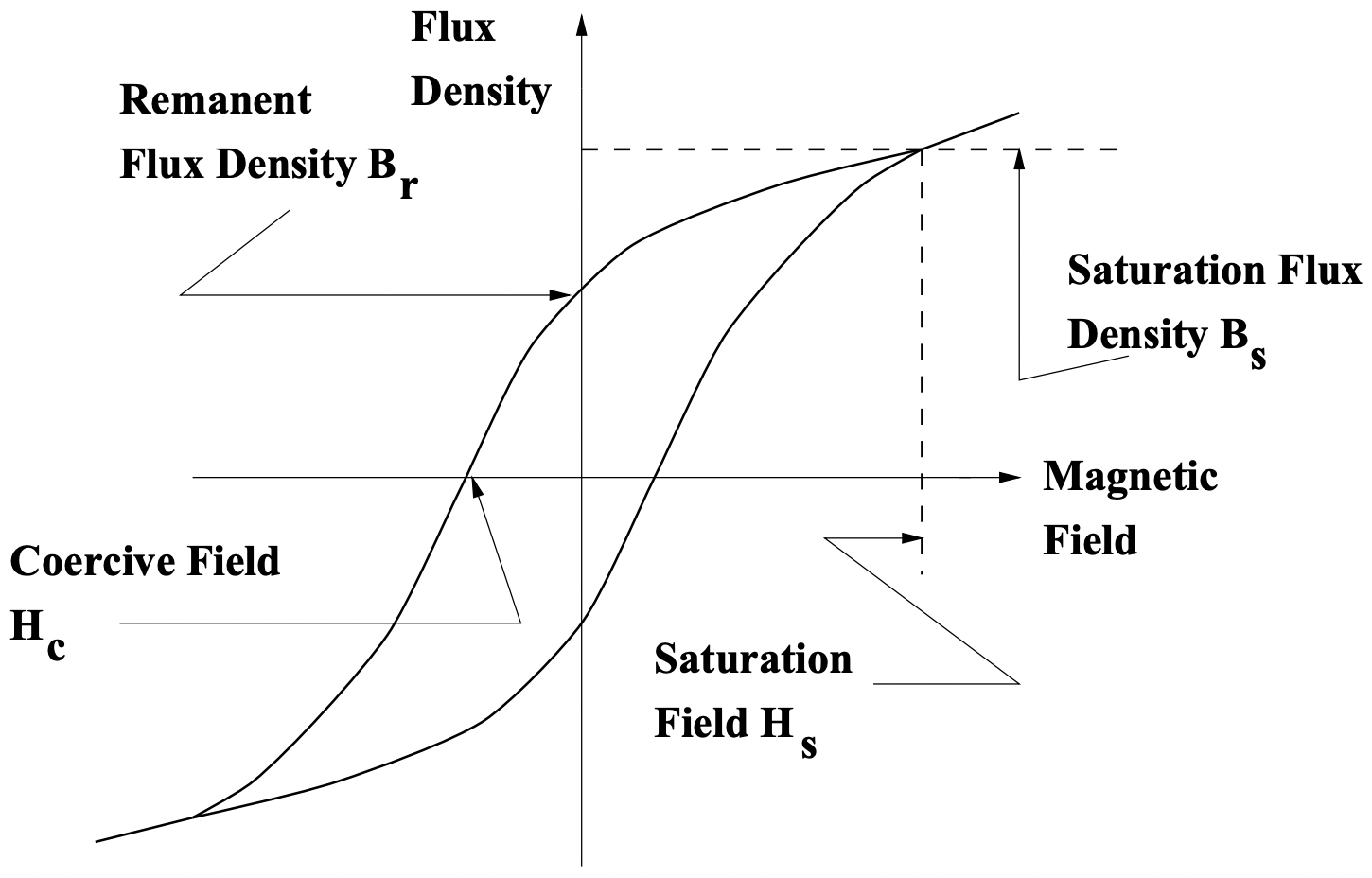Figure 10: Hysteresis Curve Nomenclature

material for which we can characterize an MMF and a flux:

\(\ \begin{aligned}
F &=N I=\int \vec{H} \cdot d e \vec{ll} \\
\Phi &=\int \frac{V}{N} d t=\iint_{\text {Area }} \vec{B} \cdot d \vec{A}
\end{aligned}\)

Energy input to the chunk of material over some period of time is

\(\ w=\int V I d t=\int F d \Phi=\int_{t} \int \vec{H} \cdot d \vec{\ell} \iint d \vec{B} \cdot d \vec{A} d t\)

Now, imagine carrying out the second (double) integral over a continuous set of surfaces which are perpendicular to the magnetic field H. (This IS possible!). The energy becomes:

\(\ w=\int_{t} \iiint \vec{H} \cdot d \vec{B} d \mathrm{vol} d t\)

and, done over a complete cycle of some input waveform, that is:

\(\ \begin{aligned}
w &=\iiint_{\mathrm{vol}} W_{m} d \mathrm{vol} \\
W_{m} &=\oint_{t} \vec{H} \cdot d \vec{B}
\end{aligned}\)

That last expression simply expresses the area of the hysteresis loop for the particular cycle.

Generally, for most electric machine applications we will use magnetic material characterized as “soft”, having as narrow a hysteresis loop (and therefore as low a hysteretic loss) as possible. At the other end of the spectrum are “hard” magnetic materials which are used to make permanent magnets. The terminology comes from steel, in which soft, annealed steel material tends to have narrow loops and hardened steel tends to have wider loops. However permanent magnet technology has advanced to the point where the coercive forces possible in even cheap ceramic magnets far exceed those of the hardest steels.

Conduction, Eddy Currents and Laminations:

Steel, being a metal, is an electrical conductor. Thus when time varying magnetic fields pass through it they cause eddy currents to flow, and of course those produce dissipation. In fact, for almost all applications involving “soft” iron, eddy currents are the dominant source of loss. To reduce the eddy current loss, magnetic circuits of transformers and electric machines are almost invariably laminated, or made up of relatively thin sheets of steel. To further reduce losses the steel is alloyed with elements (often silicon) which poison the electrical conductivity.

There are several approaches to estimating the loss due to eddy currents in steel sheets and in the surface of solid iron, and it is worthwhile to look at a few of them. It should be noted that this is a “hard” problem, since the behavior of the material itself is difficult to characterize.

Complete Penetration Case

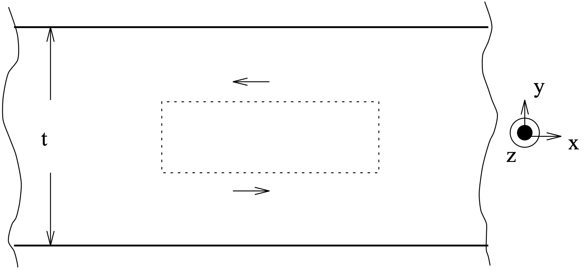Figure 11: Lamination Section for Loss Calculation

Consider the problem of a stack of laminations. In particular, consider one sheet in the stack represented in Figure 11. It has thickness \(\ t\) and conductivity \(\ \sigma\). Assume that the “skin depth” is much greater than the sheet thickness so that magnetic field penetrates the sheet completely. Further, assume that the applied magnetic flux density is parallel to the surface of the sheets:

\(\ \vec{B}=\vec{i}_{z} \operatorname{Re}\left\{\sqrt{2} B_{0} e^{j \omega t}\right\}\)

Now we can use Faraday’s law to determine the electric field and therefore current density in the sheet. If the problem is uniform in the x- and z- directions,

\(\ \frac{\partial \underline{E}_{x}}{\partial y}=-j \omega_{0} B_{0}\)

Note also that, unless there is some net transport current in the x- direction, E must be antisymmetric about the center of the sheet. Thus if we take the origin of y to be in the center, electric field and current are:

\(\ \begin{aligned}
E_{x} &=-j \omega B_{0} y \\
\underline{J}_{x} &=-j \omega B_{0} \sigma y
\end{aligned}\)

Local power dissipated is

\(\ P(y)=\omega^{2} B_{0}^{2} \sigma y^{2}=\frac{|J|^{2}}{\sigma}\)

To find average power dissipated we integrate over the thickness of the lamination:

\(\ <P>=\frac{2}{t} \int_{0}^{\frac{t}{2}} P(y) d y=\frac{2}{t} \omega^{2} B_{0}^{2} \sigma \int_{0}^{\frac{t}{2}} y^{2} d y=\frac{1}{12} \omega^{2} B_{0}^{2} t^{2} \sigma\)

Pay attention to the orders of the various terms here: power is proportional to the square of flux density and to the square of frequency. It is also proportional to the square of the lamination thickness (this is average volume power dissipation).

As an aside, consider a simple magnetic circuit made of this material, with some length \(\ \ell\) and area A, so that volume of material is \(\ \ell A\). Flux lined by a coil of N turns would be:

\(\ \Lambda=N \Phi=N A B_{0}\)

and voltage is of course just \(\ V=j w L\). Total power dissipated in this core would be:

\(\ P_{c}=A \ell \frac{1}{12} \omega^{2} B_{0}^{2} t^{2} \sigma=\frac{V^{2}}{R_{c}}\)

where the equivalent core resistance is now

\(\ R_{c}=\frac{A}{\ell} \frac{12 N^{2}}{\sigma t^{2}}\)

Eddy Currents in Saturating Iron

The same geometry holds for this pattern, although we consider only the one-dimensional problem \(\ (k \rightarrow 0)\). The problem was worked by McLean and his graduate student Agarwal Equation \ref{2} Equation \ref{1}. They assumed that the magnetic field at the surface of the flat slab of material was sinusoidal in time and of high enough amplitude to saturate the material. This is true if the material has high permeability and the magnetic field is strong. What happens is that the impressed magnetic field saturates a region of material near the surface, leading to a magnetic flux density parallel to the surface. The depth of the region affected changes with time, and there is a separating surface (in the flat problem this is a plane) that moves away from the top surface in response to the change in the magnetic field. An electric field is developed to move the surface, and that magnetic field drives eddy currents in the material.

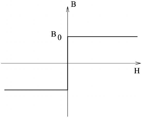Figure 12: Idealized Saturating Characteristic

Assume that the material has a perfectly rectangular magnetization curve as shown in Figure 12, so that flux density in the x- direction is:

\(\ B_{x}=B_{0} \operatorname{sign}\left(H_{x}\right)\)

The flux per unit width (in the z- direction) is:

\(\ \Phi=\int_{0}^{-\infty} B_{x} d y\)

and Faraday’s law becomes:

\(\ E_{z}=\frac{\partial \Phi}{\partial t}\)

while Ampere’s law in conjunction with Ohm’s law is:

\(\ \frac{\partial H_{x}}{\partial y}=\sigma E_{z}\)

Now, McLean suggested a solution to this set in which there is a “separating surface” at depth \(\ \zeta\) below the surface, as shown in Figure 13 . At any given time:

\(\ \begin{aligned}
H_{x} &=H_{s}(t)\left(1+\frac{y}{\zeta}\right) \\
J_{z} &=\sigma E_{z}=\frac{H_{s}}{\zeta}
\end{aligned}\)

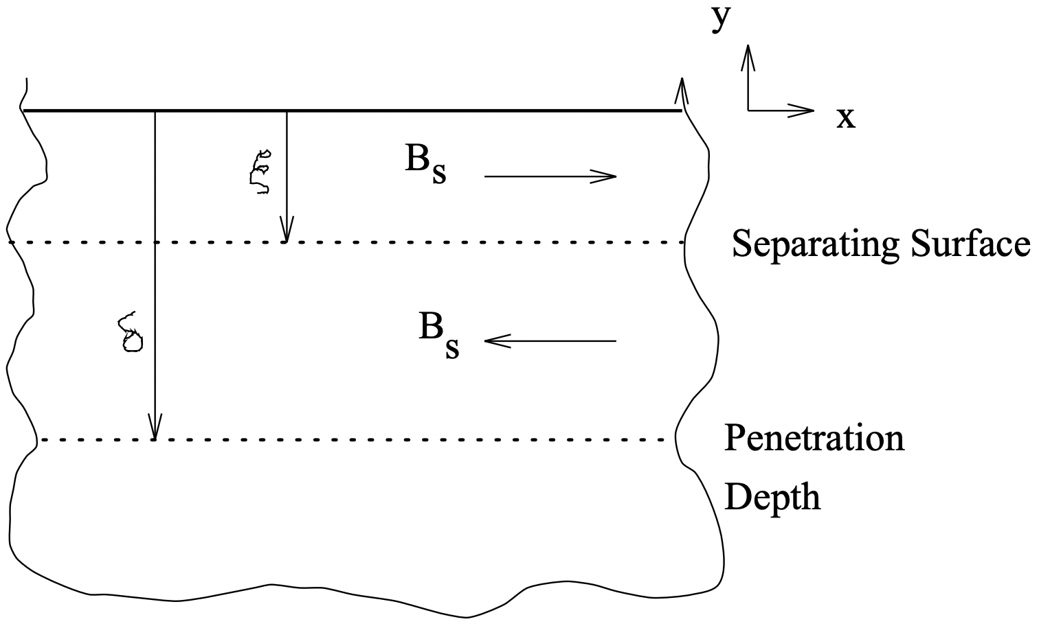Figure 13: Separating Surface and Penetration Depth

That is, in the region between the separating surface and the top of the material, electric field \(\ E_{z}\) is uniform and magnetic field \(\ H_{x}\) is a linear function of depth, falling from its impressed value at the surface to zero at the separating surface. Now: electric field is produced by the rate of change of flux which is:

\(\ E_{z}=\frac{\partial \Phi}{\partial t}=2 B_{x} \frac{\partial \zeta}{\partial t}\)

Eliminating E, we have:

\(\ 2 \zeta \frac{\partial \zeta}{\partial t}=\frac{H_{s}}{\sigma B_{x}}\)

and then, if the impressed magnetic field is sinusoidal, this becomes:

\(\ \frac{d \zeta^{2}}{d t}=\frac{H_{0}}{\sigma B_{0}}|\sin \omega t|\)

This is easy to solve, assuming that \(\ \zeta=0\) at \(\ t=0\),

\(\ \zeta=\sqrt{\frac{2 H_{0}}{\omega \sigma B_{0}}} \sin \frac{\omega t}{2}\)

Now: the surface always moves in the downward direction (as we have drawn it), so at each half cycle a new surface is created: the old one just stops moving at a maximum position, or penetration depth:

\(\ \delta=\sqrt{\frac{2 H_{0}}{\omega \sigma B_{0}}}\)

This penetration depth is analogous to the “skin depth” of the linear theory. However, it is an absolute penetration depth.

The resulting electric field is:

\(\ E_{z}=\frac{2 H_{0}}{\sigma \delta} \cos \frac{\omega t}{2} \quad 0<\omega t<\pi\)

This may be Fourier analyzed: noting that if the impressed magnetic field is sinusoidal, only the time fundamental component of electric field is important, leading to:

\(\ E_{z}=\frac{8}{3 \pi} \frac{H_{0}}{\sigma \delta}(\cos \omega t+2 \sin \omega t+\ldots)\)

Complex surface impedance is the ratio between the complex amplitude of electric and magnetic field, which becomes:

\(\ \underline{Z}_{s}=\frac{\underline{\underline{E}_{z}}}{\underline{H}_{x}}=\frac{8}{3 \pi} \frac{1}{\sigma \delta}(2+j)\)

Thus, in practical applications, we can handle this surface much as we handle linear conductive surfaces, by establishing a skin depth and assuming that current flows within that skin depth of the surface. The resistance is modified by the factor of \(\ \frac{16}{3 \pi}\) and the “power factor” of this surface is about 89 % (as opposed to a linear surface where the “power factor” is about 71 %.

Agarwal suggests using a value for \(\ B_{0}\) of about 75 % of the saturation flux density of the steel.