8.6: Semi-Empirical Method of Handling Iron Loss
- Page ID
- 55724

Neither of the models described so far are fully satisfactory in describing the behavior of laminated iron, because losses are a combination of eddy current and hysteresis losses. The rather simple model employed for eddy currents is precise because of its assumption of abrupt saturation. The hysteresis model, while precise, would require an empirical determination of the size of the hysteresis loops anyway. So we must often resort to empirical loss data. Manufacturers of lamination steel sheets will publish data, usually in the form of curves, for many of their products. Here are a few ways of looking at the data.
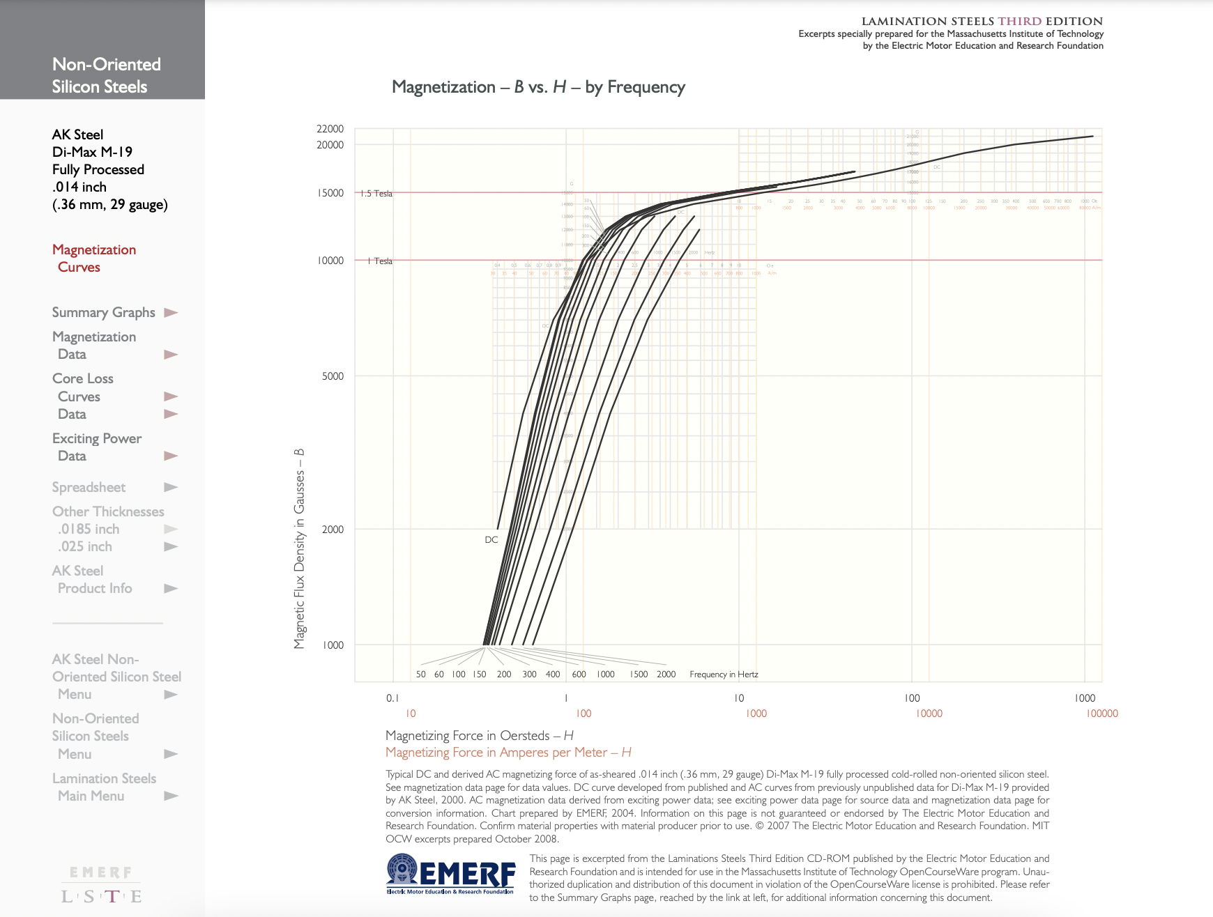
A low frequency flux density vs. magnetic field (“saturation”) curve was shown in Figure 9. Included with that was a measure of the incremental permeability
\(\ \mu^{\prime}=\frac{d B}{d H}\)
In some machine applications either the “total” inductance (ratio of flux to MMF) or “incremental” inductance (slope of the flux to MMF curve) is required. In the limit of low frequency these numbers may be useful.
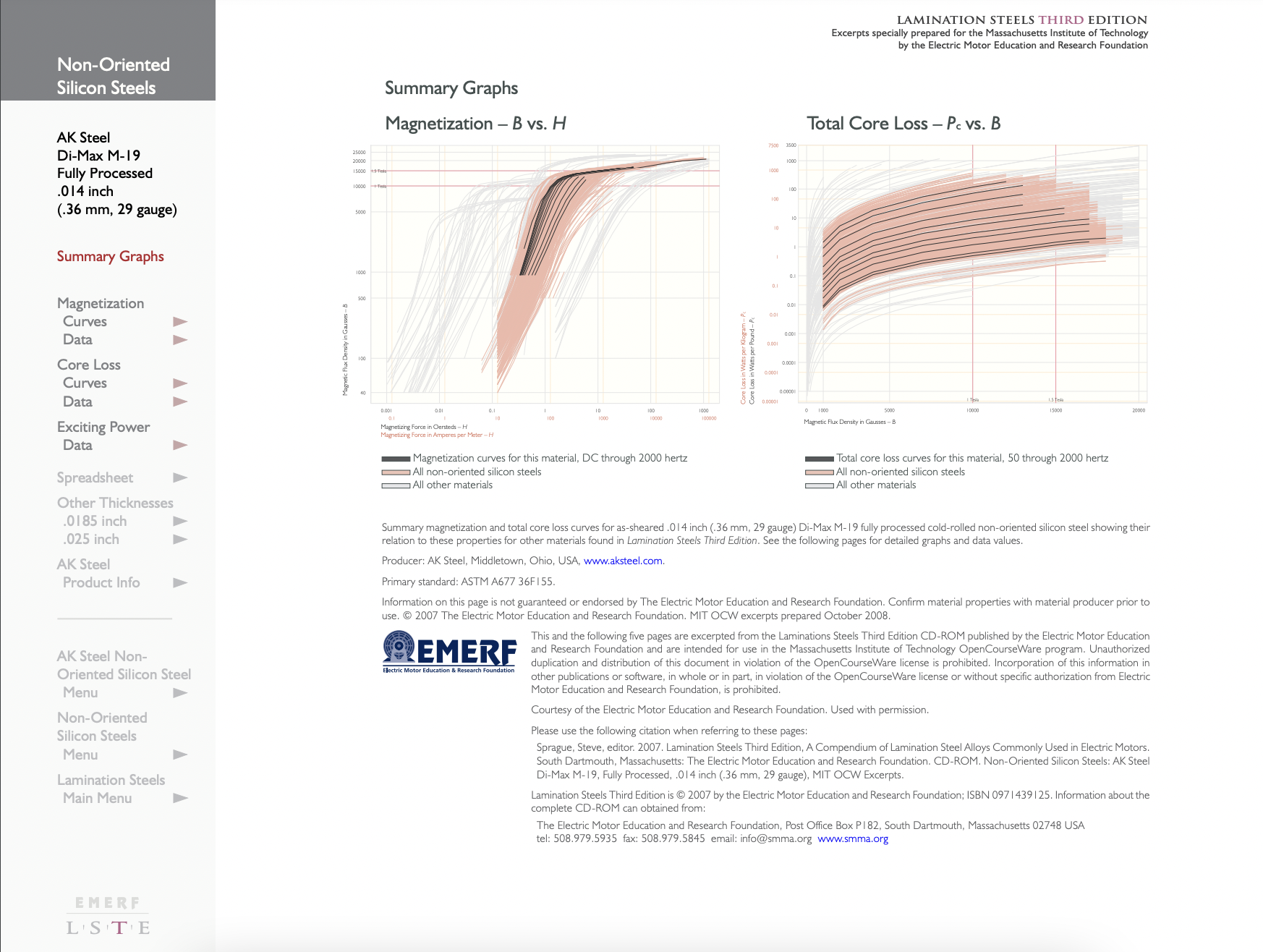
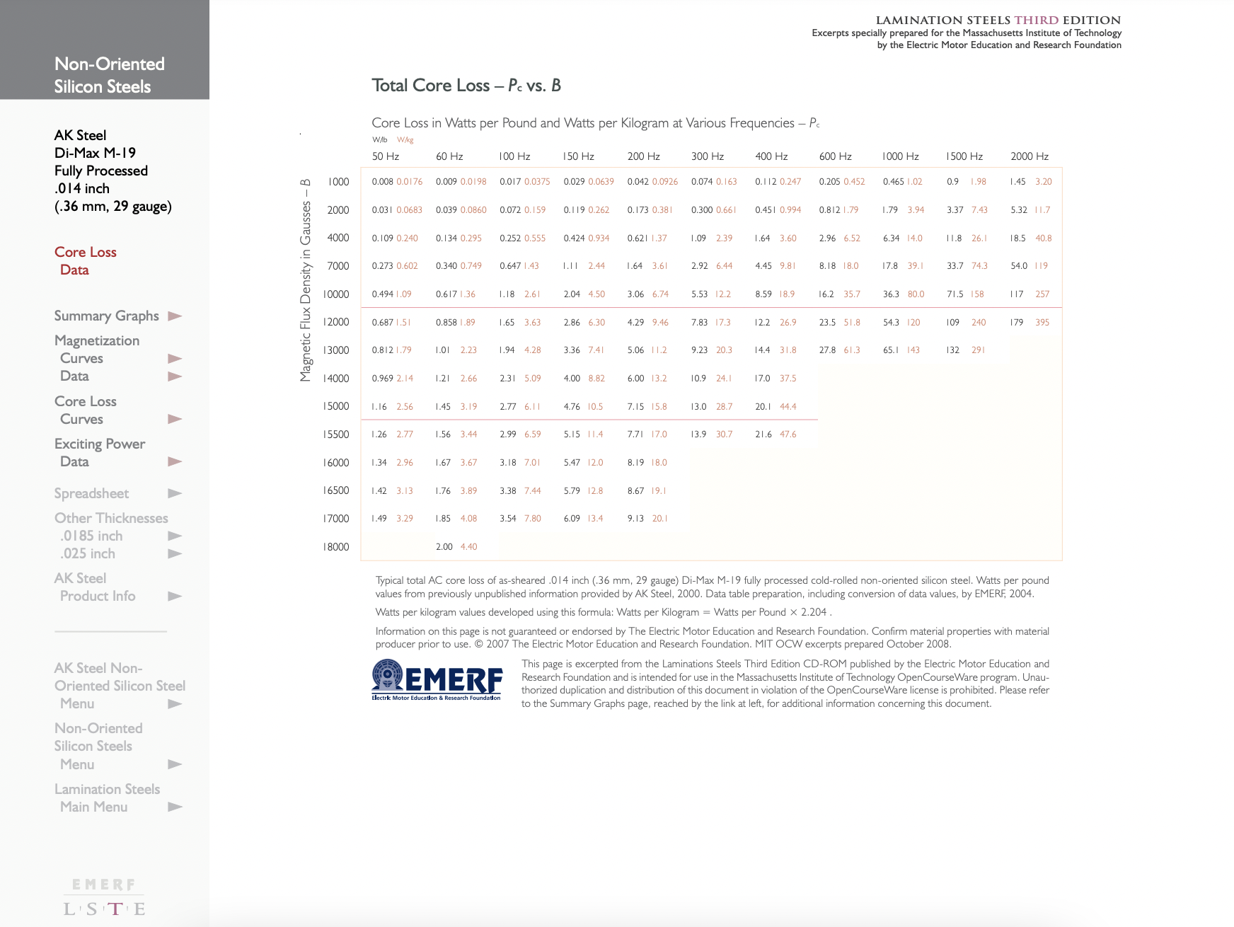
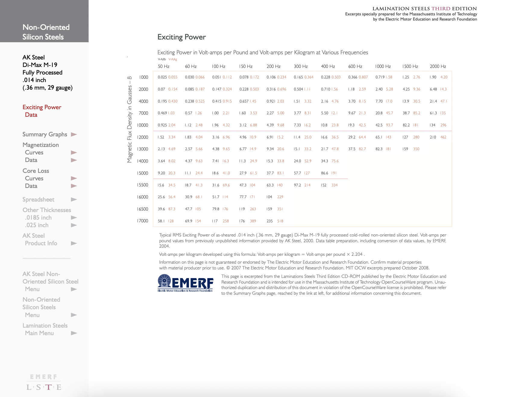
For designing electric machines, however, a second way of looking at steel may be more useful. This is to measure the real and reactive power as a function of magnetic flux density and (sometimes) frequency. In principal, this data is immediately useful. In any well-designed electric machine the flux density in the core is distributed fairly uniformly and is not strongly affected by eddy currents, etc. in the core. Under such circumstances one can determine the flux density in each part of the core. With that information one can go to the published empirical data for real and reactive power and determine core loss and reactive power requirements.
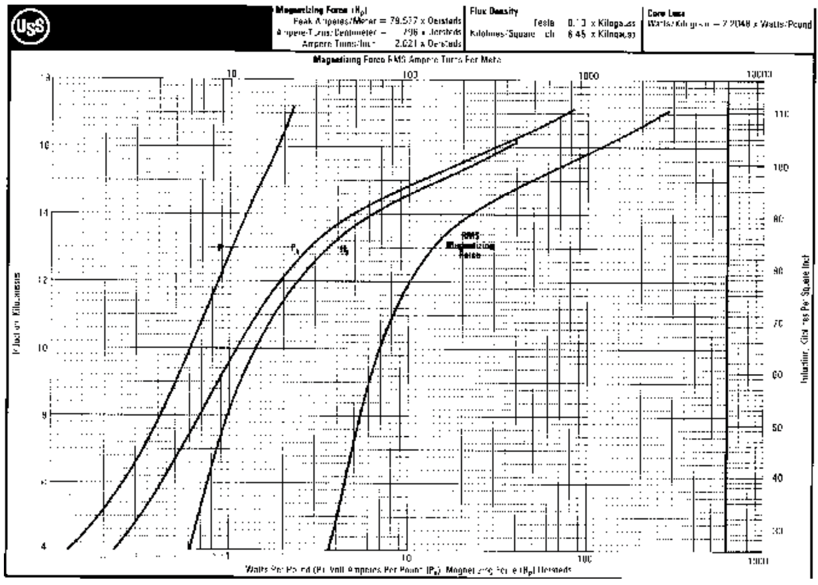
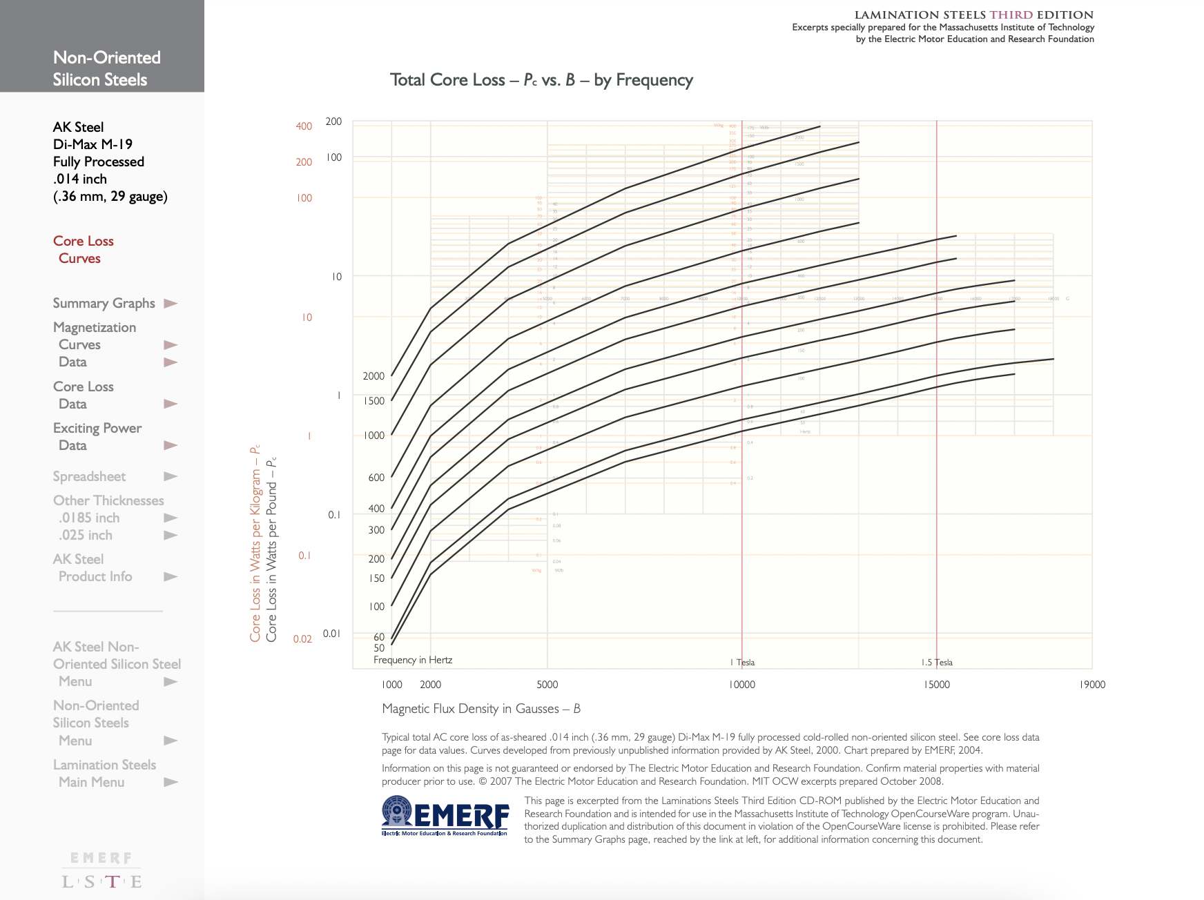
Figure 14 shows core loss and “apparent” power per unit mass as a function of (RMS) induction for 29 gage, fully processed M-19 steel. The two left-hand curves are the ones we will find most useful. "\(\ P\)" denotes real power while "\(\ P_{a}\)" denotes “apparent power”. The use of this data is quite straightforward. If the flux density in a machine is estimated for each part of the machine and the mass of steel calculated, then with the help of this chart a total core loss and apparent power can
| M-19 | M-36 | ||
| Base Flux Density | \(\ B_{0}\) | 1 T | 1 T |
| Base Frequency | \(\ f_{0}\) | 60 Hz | 60 Hz |
| Base Power (w/lb) | \(\ P_{0}\) | 0.59 | 0.67 |
| Flux Exponent | \(\ \epsilon_{B}\) | 1.88 | 1.86 |
| Frequency Exponent | \(\ \epsilon_{F}\) | 1.53 | 1.48 |
| Base Apparent Power 1 | \(\ V A_{0}\) | 1.08 | 1.33 |
| Base Apparent Power 2 | \(\ V A_{1}\) | .0144 | .0119 |
| Flux Exponent | \(\ \epsilon_{0}\) | 1.70 | 2.01 |
| Flux Exponent | \(\ \epsilon_{1}\) | 16.1 | 17.2 |
be estimated. Then the effect of the core may be approximated with a pair of elements in parallel with the terminals, with:
\(\ \begin{aligned}
R_{c} &=\frac{q|V|^{2}}{P} \\
X_{c} &=\frac{q|V|^{2}}{Q} \\
Q &=\sqrt{P_{a}^{2}-P^{2}}
\end{aligned}\)
Where \(\ q\) is the number of machine phases and \(\ V\) is phase voltage. Note that this picture is, strictly speaking, only valid for the voltage and frequency for which the flux density was calculated. But it will be approximately true for small excursions in either voltage or frequency and therefore useful for estimating voltage drop due to exciting current and such matters. In design program applications these parameters can be re-calculated repeatedly if necessary.
“Looking up” this data is a it awkward for design studies, so it is often convenient to do a “curve fit” to the published data. There are a large number of possible ways of doing this. One method that has bee found to work reasonably well for silicon iron is an “exponential fit”:
\(\ P \approx P_{0}\left(\frac{B}{B_{0}}\right)^{\epsilon_{B}}\left(\frac{f}{f_{0}}\right)^{\epsilon_{F}}\)
This fit is appropriate if the data appears on a log-log plot to lie in approximately straight lines. Figure 15 shows such a fit for the same steel sheet as the other figures.
For “apparent power” the same sort of method can be used. It appears, however, that the simple exponential fit which works well for real power is inadequate, at least if relatively high inductions are to be used. This is because, as the steel saturates, the reactive component of exciting current rises rapidly. I have had some success with a “double exponential” fit:
\(\ V A \approx V A_{0}\left(\frac{B}{B_{0}}\right)^{\epsilon_{0}}+V A_{1}\left(\frac{B}{B_{0}}\right)^{\epsilon_{1}}\)
To first order the reactive component of exciting current will be linear in frequency.
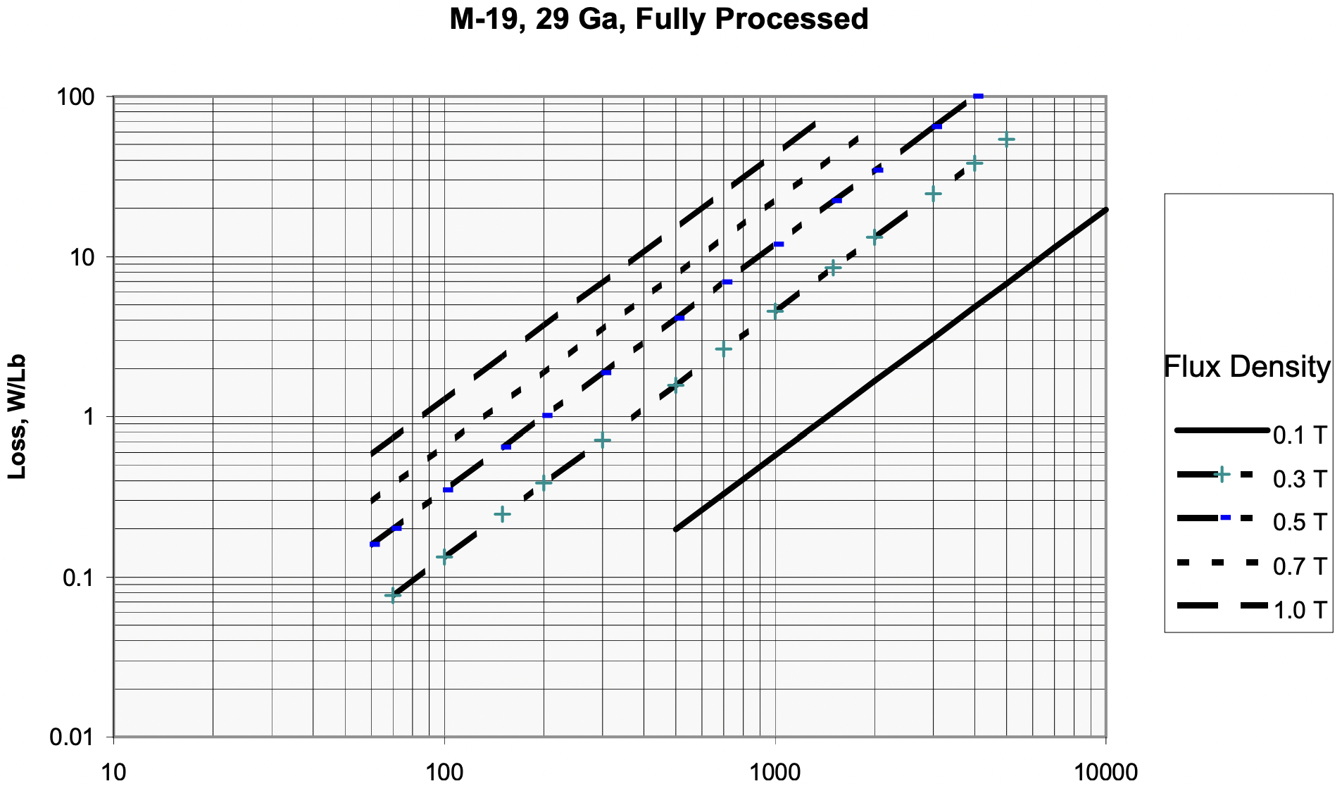 Figure 15: Steel Sheet Core Loss Fit vs. Flux Density and Frequency
In the disk that is to be distributed with these notes there are a number of data files representing properties of different types of nonoriented sheet steel. The format of each of the files is the same: two columns of numbers, the first is flux density in Tesla, RMS, 60 Hz. The second column is watts per pound or vo ). Proc is “f” for fully processed and “s” for semiprocessed. Data is “p” for power, “pa” for apparent power. Gage is 29 (.014” thick), 26 (.0185” thick) or 24 (.025” thick). Example: m19fp29.prn designates loss in M-19 material, fully processed, 29 gage.
Also on the disk are three curve fitting routines that appear to work with this data. (Not all of the routines work with all of the data!). They are:
efit <return>.fit what (name.prn) ==>Enter the file name for the material designator without the
.prnextension. The program will think about the problem for a few seconds and put up a plot of its fit with points noting the actual data. Enter a<return>and a summary of the fit turns up, including the fit parameters and an error indication. These programs use MATLAB’s fmins routine to minimize a mean-squared error as calculated by the auxiliary functionfiterr.m.e2fit.mimplements the double exponential fit of apparent power against flux density. Use is just like efit. It uses the auxiliary functionfit2err.m.pfit.muses the MATLAB function polyfit to fit a polynomial (in B) to the data.
Most of the machine design scripts enclosed with the material for this special summer subject employ the exponential fits for core iron developed here.
References
Equation \ref{1} W. MacLean, “Theory of Strong Electromagnetic Waves in Massive Iron”, Journal of Applied Physics, V.25, No 10, October, 1954
Equation \ref{2} P.D. Agarwal, “Eddy-Current Losses in Solid and Laminated Iron”, Trans. AIEE, V. 78, pp 169-171, 1959