9.6: Balanced Operation

Now, suppose the machine is operated in this fashion: the rotor turns at a constant velocity, the field current is held constant, and the three stator currents are sinusoids in time, with the same amplitude and with phases that differ by 120 degrees.

\(\ \begin{aligned}
p \phi &=\omega t+\delta_{i} \\
i_{f} &=I_{f} \\
i_{a} &=I \cos (\omega t) \\
i_{b} &=I \cos \left(\omega t-\frac{2 \pi}{3}\right) \\
i_{c} &=I \cos \left(\omega t+\frac{2 \pi}{3}\right)
\end{aligned}\)

Straightforward (but tedious) manipulation yields an expression for torque:

\(\ T=-\frac{3}{2} p M I I_{f} \sin \delta_{i}\)

Operated in this way, with balanced currents and with the mechanical speed consistent with the electrical frequency \(\ (p \Omega=\omega)\), the machine exhibits a constant torque. The phase angle \(\ \delta_{i}\) is called the torque angle, but it is important to use some caution, as there is more than one torque angle.

Now, look at the machine from the electrical terminals. Flux linked by Phase A will be:

\(\ \lambda_{a}=L_{a} i_{a}+L_{a b} i_{b}+L_{a c} i_{c}+M I_{f} \cos p \phi\)

Noting that the sum of phase currents is, under balanced conditions, zero and that the mutual phase-phase inductances are equal, this simplifies to:

\(\ \lambda_{a}=\left(L_{a}-L_{a b}\right) i_{a}+M I_{f} \cos p \phi=L_{d} i_{a}+M I_{f} \cos p \phi\)

where we use the notation \(\ L_{d}\) to denote synchronous inductance.

Now, if the machine is turning at a speed consistent with the electrical frequency we say it is operating synchronously, and it is possible to employ complex notation in the sinusoidal steady state. Then, note:

\(\ i_{a}=I \cos \left(\omega t+\theta_{i}\right)=\operatorname{Re}\left\{I e^{j \omega t+\theta_{i}}\right\}\)

If , we can write an expression for the complex amplitude of flux as:

\(\ \lambda_{a}=\operatorname{Re}\left\{\underline{\Lambda}_{a} e^{j \omega t}\right\}\)

where we have used this complex notation:

\(\ \begin{aligned}
\underline{I} &=I e^{j \theta_{i}} \\
\underline{I}_{f} &=I_{f} e^{j \theta_{m}}
\end{aligned}\)

Now, if we look for terminal voltage of this system, it is:

\(\ v_{a}=\frac{d \lambda_{a}}{d t}=\operatorname{Re}\left\{j \omega \underline{\Lambda}_{a} e^{j \omega t}\right\}\)

This system is described by the equivalent circuit shown in Figure 2.

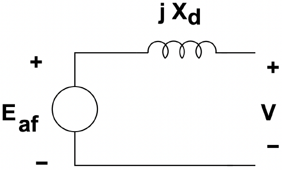Figure 2: Round Rotor Synchronous Machine Equivalent Circuit

where the internal voltage is:

\(\ \underline{E}_{a f}=j \omega M I_{f} e^{j \theta_{m}}\)

Now, if that is connected to a voltage source (i.e. if is fixed), terminal current is:

\(\ \underline{I}=\frac{\underline{V}-E_{a f} e^{j \delta}}{j X_{d}}\)

where \(\ X_{d}=\omega L_{d}\) is the synchronous reactance.

Then real and reactive power (in phase A) are:

\(\ \begin{aligned}
P+j Q &=\frac{1}{2} \underline{V I^{*}} \\
&=\frac{1}{2} \underline{V}\left(\frac{\underline{V}-E_{a f} e^{j \delta}}{j X_{d}}\right)^{*} \\
&=\frac{1}{2} \frac{|\underline{V}|^{2}}{-j X_{d}}-\frac{1}{2} \frac{V E_{a f} e^{j \delta}}{-j X_{d}}
\end{aligned}\)

This makes real and reactive power:

\(\ \begin{aligned}
P_{a} &=-\frac{1}{2} \frac{V E_{a f}}{X_{d}} \sin \delta \\
Q_{a} &=\frac{1}{2} \frac{V^{2}}{X_{d}}-\frac{1}{2} \frac{V E_{a f} X_{d}}{\cos } \delta
\end{aligned}\)

If we consider all three phases, real power is

\(\ P=-\frac{3}{2} \frac{V E_{a f}}{X_{d}} \sin \delta\)

Now, at last we need to look at actual operation of these machines, which can serve either as motors or as generators.

Vector diagrams that describe operation as a motor and as a generator are shown in Figures 3 and 4, respectively.

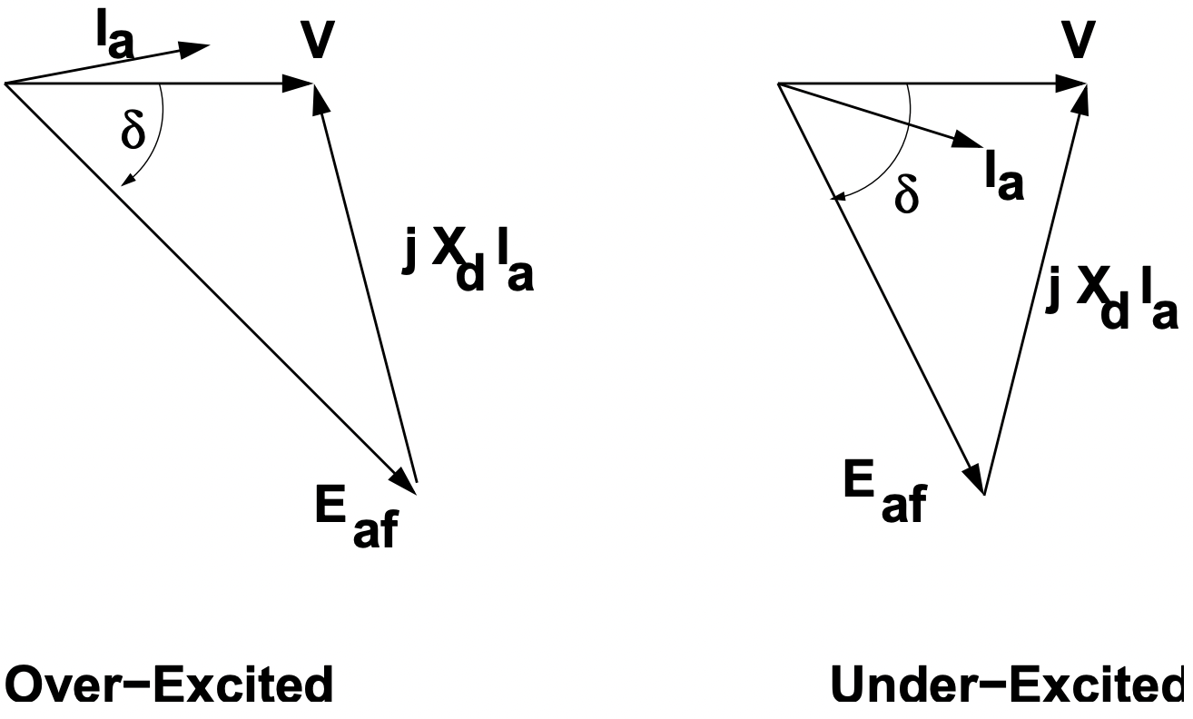Figure 3: Motor Operation, Under- and Over- Excited

Operation as a generator is not much different from operation as a motor, but it is common to make notations with the terminal current given the opposite (“generator”) sign.

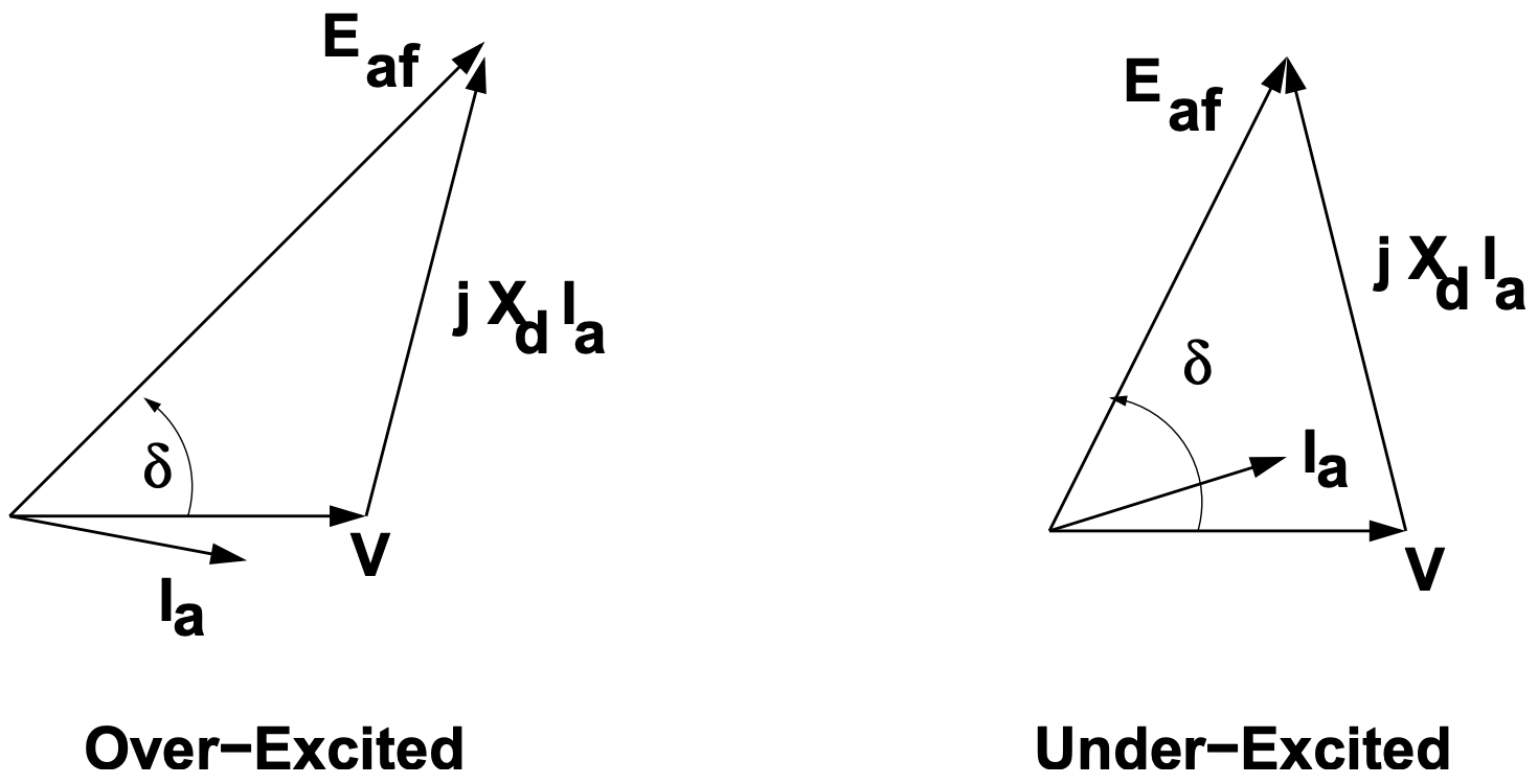Figure 4: Generator Operation, Under- and Over- Excited