9.7: Reconciliation of Models

We have determined that we can predict its power and/or torque characteristics from two points of view : first, by knowing currents in the rotor and stator we could derive an expression for torque vs. a power angle:

\(\ T=-\frac{3}{2} p M I I_{f} \sin \delta_{i}\)

From a circuit point of view, it is possible to derive an expression for power:

\(\ P=-\frac{3}{2} \frac{V E_{a f}}{X_{d}} \sin \delta\)

and of course since power is torque times speed, this implies that:

\(\ T=-\frac{3}{2} \frac{V E_{a f}}{\Omega X_{d}} \sin \delta=-\frac{3}{2} \frac{p V E_{a f}}{\omega X_{d}} \sin \delta\)

In this section of the notes we will, first of all, reconcile these notions, look a bit more at what they mean, and then generalize our simple theory to salient pole machines as an introduction to two-axis theory of electric machines.

Torque Angles:

Figure 5 shows a vector diagram that shows operation of a synchronous motor. It represents the MMF’s and fluxes from the rotor and stator in their respective positions in space during normal operation. Terminal flux is chosen to be ‘real’, or occupy the horizontal position. In motor operation the rotor lags by angle \(\ \delta\), so the rotor flux \(\ M I_{f}\) is shown in that position. Stator current is also shown, and the torque angle between it and the rotor, \(\ \delta_{i}\) is also shown. Now, note that the dotted line OA, drawn perpendicular to a line drawn between the stator flux \(\ L_{d} I\) and terminal flux \(\ \Lambda_{t}\), has length:

\(\ |O A|=L_{d} I \sin \delta_{i}=\Lambda_{t} \sin \delta\)

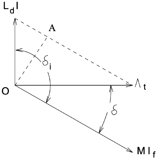Figure 5: Synchronous Machine Phasor Addition

Then, noting that terminal voltage \(\ V=\omega \Lambda_{t}\), \(\ E_{a}=\omega M I_{f}\) and \(\ X_{d}=\omega L_{d}\), straightforward substitution yields:

\(\ \frac{3}{2} \frac{p V E_{a f}}{\omega X_{d}} \sin \delta=\frac{3}{2} p M I I_{f} \sin \delta_{i}\)

So the current- and voltage- based pictures do give the same result for torque.