9.9: Normal Operation

The synchronous machine is used, essentially interchangeably, as a motor and as a generator. Note that, as a motor, this type of machine produces torque only when it is running at synchronous speed. This is not, of course, a problem for a turbogenerator which is started by its prime mover (e.g. a steam turbine). Many synchronous motors are started as induction machines on their damper cages (sometimes called starting cages). And of course with power electronic drives the machine can often be considered to be “in synchronism” even down to zero speed.

As either a motor or as a generator, the synchronous machine can either produce or consume reactive power. In normal operation real power is dictated by the load (if a motor) or the prime mover (if a generator), and reactive power is determined by the real power and by field current.

Figure 6 shows one way of representing the capability of a synchronous machine. This picture represents operation as a generator, so the signs of \(\ p\) and \(\ q\) are reversed, but all of the other elements of operation are as we ordinarily would expect. If we plot \(\ p\) and \(\ q\) (calculated in the normal way) against each other, we see the construction at the right. If we start at a location \(\ q=-v^{2} / x_{d}\), (and remember that normally \(\ v=1\) per-unit , then the locus of \(\ p\) and \(\ q\) is what would be obtained by swinging a vector of length \(\ v e_{a f} / x_{d}\) over an angle \(\ \delta\). This is called a capability chart because it is an easy way of visualizing what the synchronous machine (in this case generator) can do. There are three easily noted limits to capability. The upper limit is a circle (the one traced out by that vector) which is referred to as field capability. The second limit is a circle that describes constant \(\ |p+j q|\). This is, of course, related to the magnitude of armature current and so this limit is called armature capability. The final limit is related to machine stability, since the torque angle cannot go beyond 90 degrees. In actuality there are often other limits that can be represented on this type of a chart. For example, large synchronous generators typically have a problem with heating of the

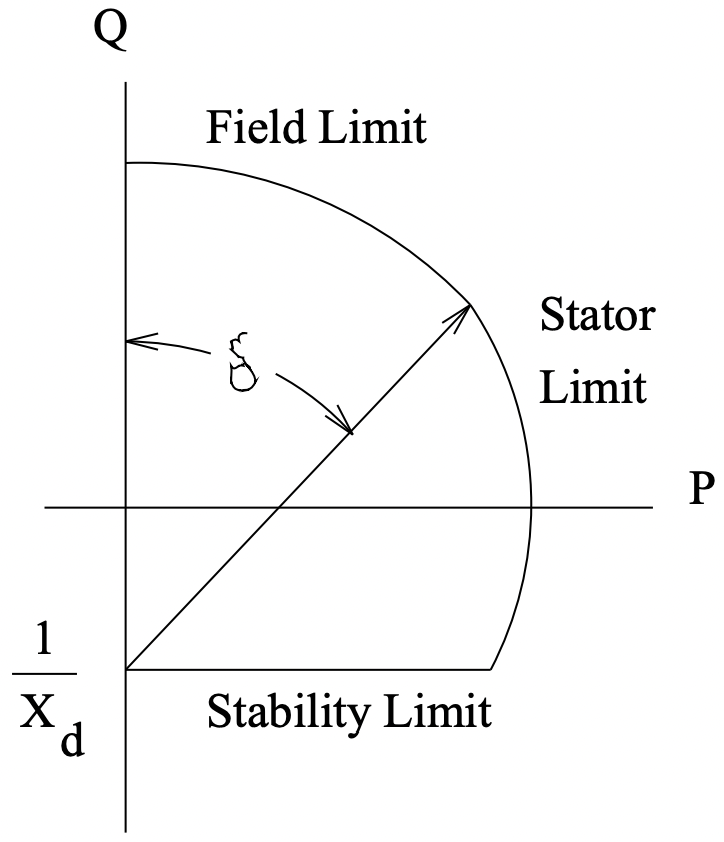Figure 6: Synchronous Generator Capability Diagram

stator iron when they attempt to operate in highly underexcited conditions (q strongly negative), so that one will often see another limit that prevents the operation of the machine near its stability limit. In very large machines with more than one cooling state (e.g. different values of cooling hydrogen pressure) there may be multiple curves for some or all of the limits.

Another way of describing the limitations of a synchronous machine is embodied in the Vee Curve. An example is shown in Figure 7 . This is a cross-plot of magnitude of armature current with field current. Note that the field and armature current limits are straightforward (and are the right-hand and upper boundaries, respectively, of the chart). The machine stability limit is what terminates each of the curves at the upper left-hand edge. Note that each curve has a minimum at unity power factor. In fact, there is yet another cross-plot possible, called a compounding curve, in which field current is plotted against real power for fixed power factor.