9.10: Salient Pole Machines- Two-Reaction Theory

So far, we have been describing what are referred to as “round rotor” machines, in which stator reactance is not dependent on rotor position. This is a pretty good approximation for large turbine generators and many smaller two-pole machines, but it is not a good approximation for many synchronous motors nor for slower speed generators. For many such applications it is more cost effective to wind the field conductors around steel bodies (called poles) which are then fastened onto the rotor body, with bolts or dovetail joints. These produce magnetic anisotropies into the machine which affect its operation. The theory which follows is an introduction to two-reaction theory and consequently for the rotating field transformations that form the basis for most modern dynamic analyses.

Figure 8 shows a very schematic picture of the salient pole machine, intended primarily to show how to frame this analysis. As with the round rotor machine the stator winding is located in slots in the surface of a highly permeable stator core annulus. The field winding is wound around steel pole pieces. We separate the stator current sheet into two components: one aligned with and one

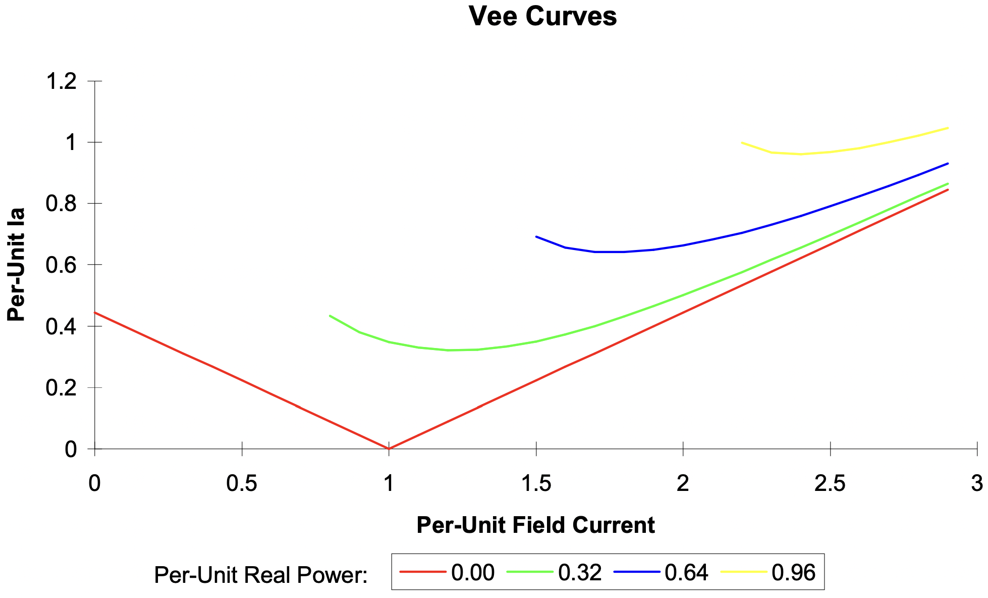Figure 7: Synchronous Machine Vee Curve

in quadrature to the field. Remember that these two current components are themselves (linear) combinations of the stator phase currents. The transformation between phase currents and the dand q- axis components is straightforward and will appear in Chapter 4 of these notes.

The key here is to separate MMF and flux into two orthogonal components and to pretend that each can be treated as sinusoidal. The two components are aligned with the direct axis and with the quadrature axis of the machine. The direct axis is aligned with the field winding, while the quadrature axis leads the direct by 90 degrees. Then, if \(\ \phi\) is the angle between the direct axis and the axis of phase a, we can write for flux linking phase a:

\(\ \lambda_{a}=\lambda_{d} \cos \phi-\lambda_{q} \sin \phi\)

Then, in steady state operation, if \(\ V_{a}=\frac{d \lambda_{a}}{d t}\), and \(\ \phi=\omega t+\operatorname{delta}\),

\(\ V_{a}=-\omega \lambda_{d} \sin \phi-\omega \lambda_{q} \cos \phi\)

which allows us to define:

\(\ \begin{array}{l}
V_{d}=-\omega \lambda_{q} \\
V_{q}=\omega \lambda_{d}
\end{array}\)

one might think of the ‘voltage’ vector as leading the ‘flux’ vector by 90 degrees.

Now, if the machine is linear, those fluxes are given by:

\(\ \begin{aligned}
\lambda_{d} &=L_{d} I_{d}+M I_{f} \\
\lambda_{q} &=L_{q} I_{q}
\end{aligned}\)

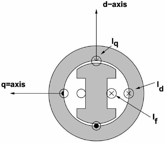Figure 8: Cartoon of a Salient Pole Synchronous Machine

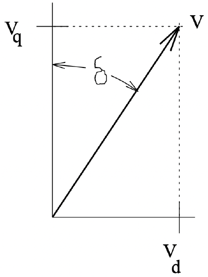Figure 9: Resolution of Terminal Voltage

Note that, in general, \(\ L_{d} \neq L_{q}\). In wound-field synchronous machines, usually \(\ L_{d}>L_{q}\). The reverse is true for most salient (buried magnet) permanent magnet machines.

Referring to Figure 9, one can resolve terminal voltage into these components:

\(\ \begin{array}{l}
V_{d}=V \sin \delta \\
V_{q}=V \cos \delta
\end{array}\)

or:

\(\ \begin{aligned}
V_{d} &=-\omega \lambda_{q}=-\omega L_{q} I_{q}=V \sin \delta \\
V_{q} &=\omega \lambda_{d}=\omega L_{d} I_{d}+\omega M I_{f}=V \cos \delta
\end{aligned}\)

which is easily inverted to produce:

\(\ \begin{aligned}
I_{d}&=\frac{V \cos \delta-E_{a f}}{X_{d}}\\
I_{q}&=-\frac{V \sin \delta}{X_{q}}
\end{aligned}\)

where

\(\ X_{d}=\omega L_{d} \quad X_{q}=\omega L_{q} \quad E_{a f}=\omega M I_{f}\)

Now, we are working in ordinary variables (this discussion should help motivate the use of perunit!), and each of these variables is peak amplitude. Then, if we take up a complex frame of reference:

\(\ \begin{aligned}
\underline{V} &=V_{d}+j V_{q} \\
\underline{I} &=I_{d}+j I_{q}
\end{aligned}\)

complex power is:

\(\ P+j Q=\frac{3}{2} \underline{V I}^{*}=\frac{3}{2}\left\{\left(V_{d} I_{d}+V_{q} I_{q}\right)+j\left(V_{q} I_{d}-V_{d} I_{q}\right)\right\}\)

or:

\(\ \begin{aligned}
P &=-\frac{3}{2}\left(\frac{V E_{a f}}{X_{d}} \sin \delta+\frac{V^{2}}{2}\left(\frac{1}{X_{d}}-\frac{1}{X_{q}}\right) \sin 2 \delta\right) \\
Q &=\frac{3}{2}\left(\frac{V^{2}}{2}\left(\frac{1}{X_{d}}+\frac{1}{X_{q}}\right)-\frac{V^{2}}{2}\left(\frac{1}{X_{d}}-\frac{1}{X_{q}}\right) \cos 2 \delta-\frac{V E_{a f}}{X_{d}} \cos \delta\right)
\end{aligned}\)

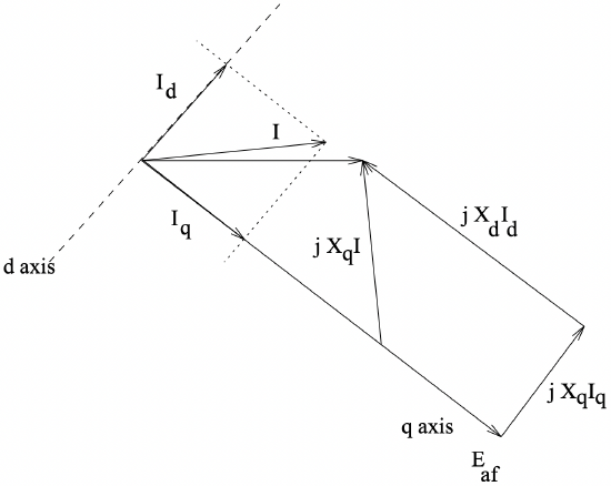Figure 10: Phasor Diagram: Salient Pole Machine

A phasor diagram for a salient pole machine is shown in Figure 10. This is a little different from the equivalent picture for a round-rotor machine, in that stator current has been separated into its d- and q- axis components, and the voltage drops associated with those components have been drawn separately. It is interesting and helpful to recognize that the internal voltage \(\ E_{a f}\) can be expressed as:

\(\ E_{a f}=E_{1}+\left(X_{d}-X_{q}\right) I_{d}\)

where the voltage \(\ E_{1}\) is on the quadrature axis. In fact, E1 would be the internal voltage of a round rotor machine with reactance \(\ X_{q}\) and the same stator current and terminal voltage. Then the operating point is found fairly easily:

\(\ \begin{aligned}
\delta &=-\tan ^{-1}\left(\frac{X_{q} I \sin \psi}{V+X_{q} I \cos \psi}\right) \\
E_{1} &=\sqrt{\left(V+X_{q} I \sin \psi\right)^{2}+\left(X_{q} I \cos \psi\right)^{2}}
\end{aligned}\)

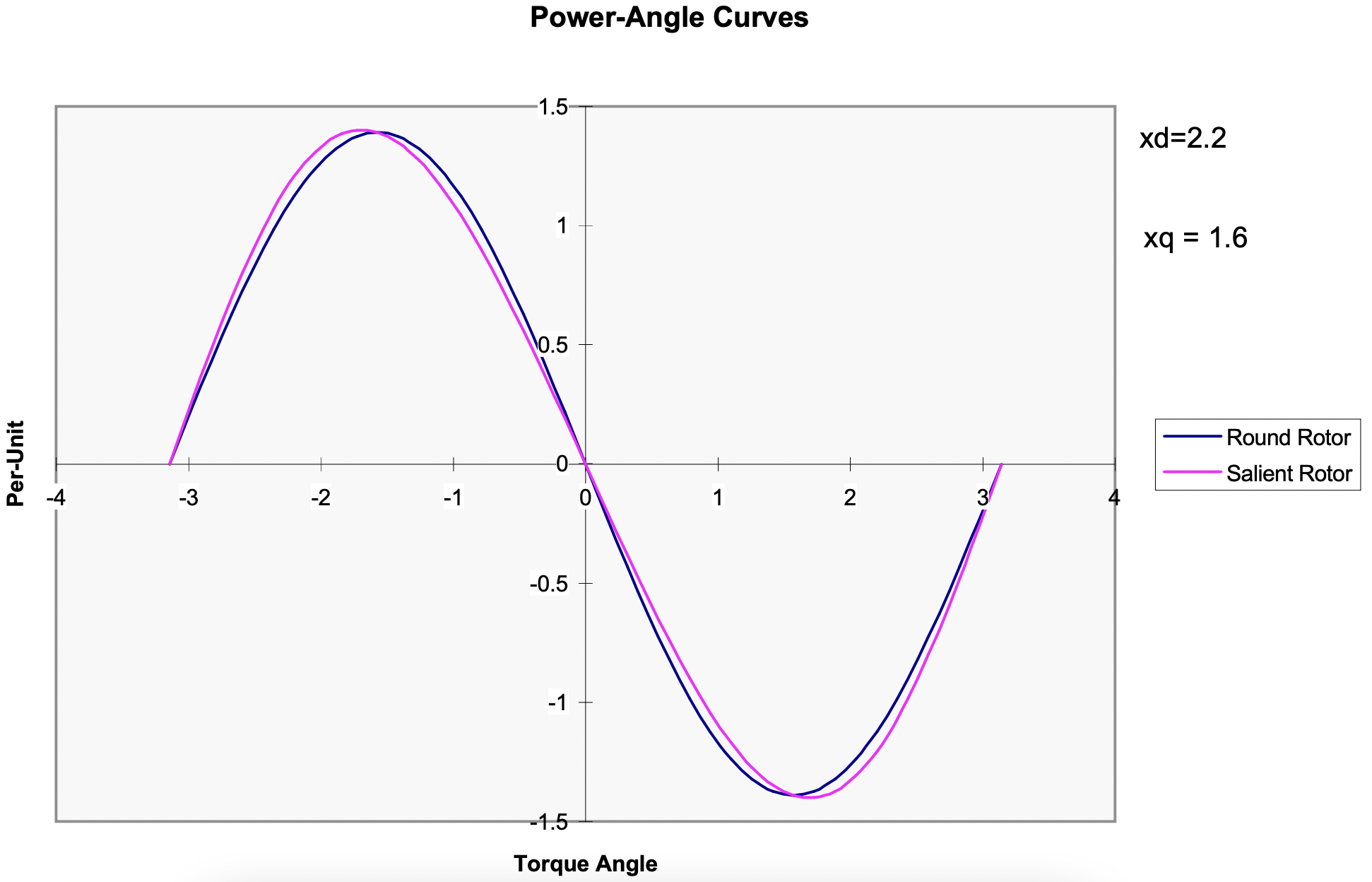Figure 11: Torque-Angle Curves: Round Rotor and Salient Pole Machines

A comparison of torque-angle curves for a pair of machines, one with a round, one with a salient rotor is shown in Figure 11 . It is not too difficult to see why power systems analysts often neglect saliency in doing things like transient stability calculations.