11.1: Introduction

Virtually all electric machines, and all practical electric machines employ some form of rotating or alternating field/current system to produce torque. While it is possible to produce a “true DC” machine (e.g. the “Faraday Disk”), for practical reasons such machines have not reached application and are not likely to. In the machines we have examined so far the machine is operated from an alternating voltage source. Indeed, this is one of the principal reasons for employing AC in power systems.

The first electric machines employed a mechanical switch, in the form of a carbon brush/commutator system, to produce this rotating field. While the widespread use of power electronics is making “brushless” motors (which are really just synchronous machines) more popular and common, commutator machines are still economically very important. They are relatively cheap, particularly in small sizes, they tend to be rugged and simple.

You will find commutator machines in a very wide range of applications. The starting motor on all automobiles is a series-connected commutator machine. Many of the other electric motors in automobiles, from the little motors that drive the outside rear-view mirrors to the motors that drive the windshield wipers are permanent magnet commutator machines. The large traction motors that drive subway trains and diesel/electric locomotives are DC commutator machines (although induction machines are making some inroads here). And many common appliances use “universal” motors: series connected commutator motors adapted to AC.

Geometry

A schematic picture (“cartoon”) of a commutator type machine is shown in 1. The armature of this machine is on the rotor (this is the part that handles the electric power), and current is fed to the armature through the brush/commutator system. The interaction magnetic field is provided

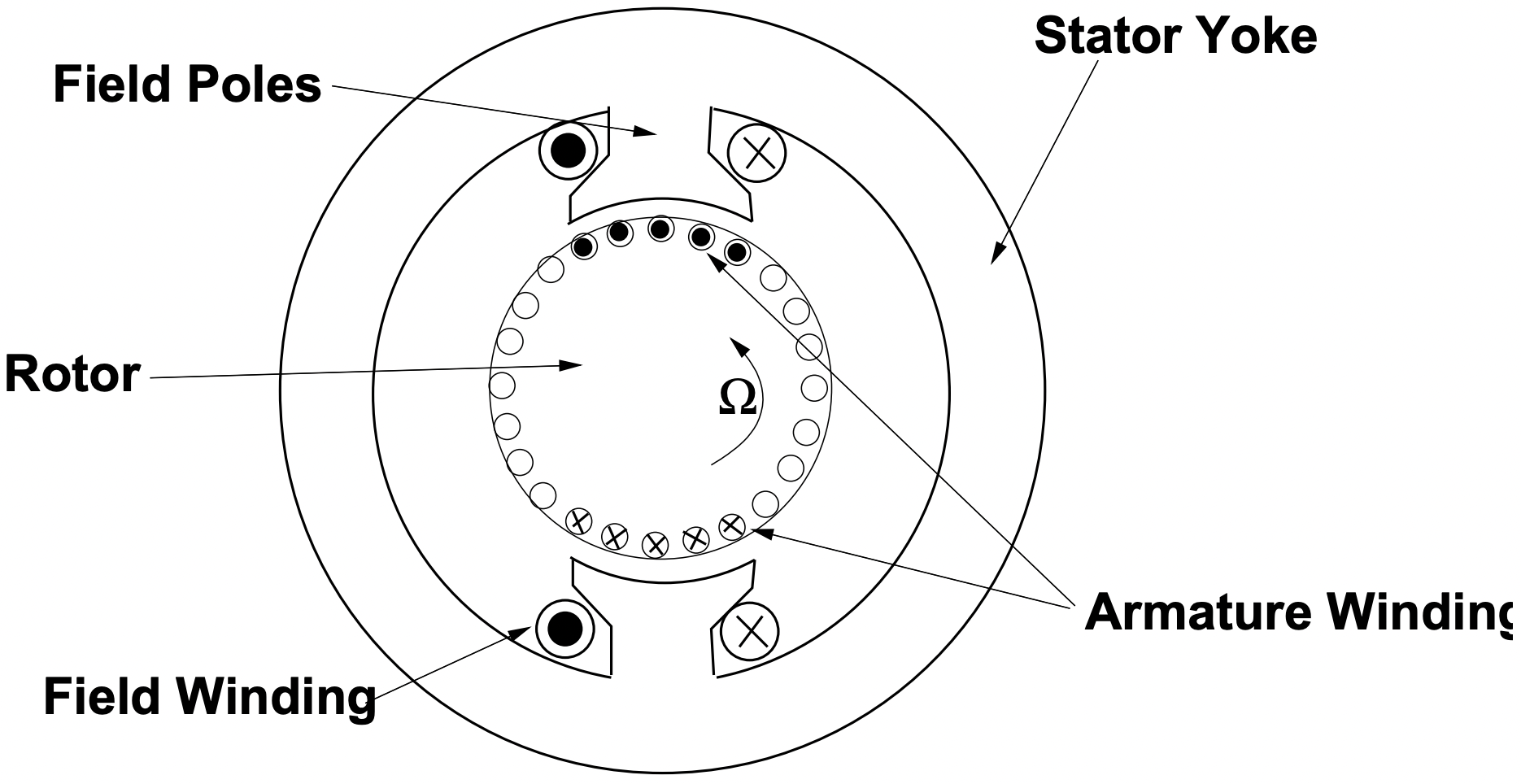Figure 1: Wound-Field DC Machine Geometry

(in this picture) by a field winding. A permanent magnet field is applicable here, and we will have quite a lot more to say about such arrangements below.

Now, if we assume that the interaction magnetic flux density averages \(\ B_{r}\), and if there are \(\ C_{a}\) conductors underneath the poles at any one time, and if there are m parallel paths, then we may estimate torque produced by the machine by:

\(\ T_{e}=\frac{C_{a}}{m} R \ell B_{r} I_{a}\)

where \(\ R\) and \(\ \ell\) are rotor radius and length, respectively and \(\ I_{a}\) is terminal current. Note that \(\ C_{a}\) is not necessarily the total number of conductors, but rather the total number of active conductors (that is, conductors underneath the pole and therefore subject to the interaction field). Now, if we note \(\ N_{f}\) as the number of field turns per pole, the interaction field is just:

\(\ B_{r}=\frac{N_{f} I_{f}}{g}\)

leading to a simple expression for torque in terms of the two currents:

\(\ T_{e}=G I_{a} I_{f}\)

where G is now the motor coefficient (units of N-m/ampere squared):

\(\ G=\mu_{0} \frac{C_{a}}{m} \frac{N_{f}}{g} R \ell\)

Now, let’s go back and look at this from the point of view of voltage. Start with Faraday’s Law:

\(\ \nabla \times \vec{E}=-\frac{\partial \vec{B}}{\partial t}\)

Integrating both sides and noting that the area integral of a curl is the edge integral of the quantity, we find:

\(\ \oint \vec{E} \cdot d \bar{\ell}=-\iint \frac{\partial \vec{B}}{\partial t}\)

Now, that is a bit awkward to use, particularly in the case we have here in which the edge of the contour is moving (note we will be using this expression to find voltage). We can make this a bit more convenient to use if we note:

\(\ \frac{d}{d t} \iint \vec{B} \cdot \vec{n} d a=\iint \frac{\partial \vec{B}}{\partial t} \cdot \vec{n} d a+\oint \vec{v} \times \vec{B} \cdot d \vec{\ell}\)

where \(\ \vec{v}\) is the velocity of the contour. This gives us a convenient way of noting the apparent electric field within a moving object (as in the conductors in a DC machine):

\(\ \vec{E}^{\prime}=\vec{E}+\vec{v} \times \vec{B}\)

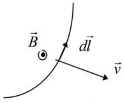Figure 2: Motion of a contour through a magnetic field produces flux change and electric field in the moving contour

Now, note that the armature conductors are moving through the magnetic field produced by the stator (field) poles, and we can ascribe to them an axially directed electric field:

\(\ E_{z}=-R \Omega B_{r}\)

If the armature conductors are arranged as described above, with \(\ C_{a}\) conductors in m parallel paths underneath the poles and with a mean active radial magnetic field of \(\ B_{r}\), we can compute a voltage induced in the stator conductors:

\(\ E_{b}=\frac{C_{a}}{m} R \Omega B_{r}\)

Note that this is only the voltage induced by motion of the armature conductors through the field and does not include brush or conductor resistance. If we include the expression for effective magnetic field, we find that the back voltage is:

\(\ E_{b}=G \Omega I_{f}\)

which leads us to the conclusion that newton-meters per ampere squared equals volt seconds per ampere. This stands to reason if we examine electric power into the interaction and mechanical power out:

\(\ P_{e m}=E_{b} I_{a}=T_{e} \Omega\)

Now, a more complete model of this machine would include the effects of armature, brush and lead resistance, so that in steady state operation:

\(\ V_{a}=R_{a} I_{a}+G \Omega I_{f}\)

Now, consider this machine with its armatucre connected to a voltage source and its field operating at steady current, so that:

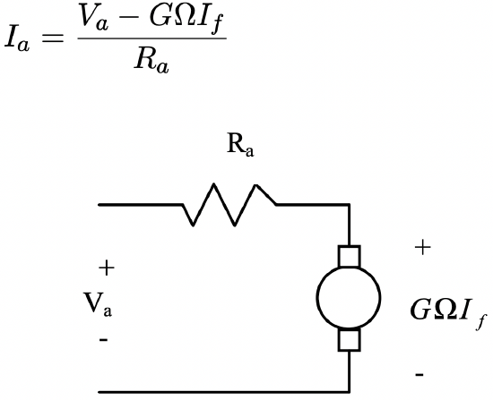Figure 3: DC Machine Equivalent Circuit

Then torque, electric power in and mechanical power out are:

\(\ \begin{aligned}
T_{e} &=G I_{f} \frac{V_{a}-G \Omega I_{f}}{R_{a}} \\
P_{e} &=V_{a} \frac{V_{a}-G \Omega I_{f}}{R_{a}} \\
P_{m} &=G \Omega I_{f} \frac{V_{a}-G \Omega I_{f}}{R_{a}}
\end{aligned}\)

Now, note that these expressions define three regimes defined by rotational speed. The two “break points” are at zero speed and at the “zero torque” speed:

\(\ \Omega_{0}=\frac{V_{a}}{G I_{f}}\)

For \(\ 0<\Omega<\Omega_{0}\), the machine is a motor: electric power in and mechanical power out are both positive. For higher speeds: \(\ \Omega_{0}<\Omega\), the machine is a generator, with electrical power in and mechanical power out being both negative. For speeds less than zero, electrical power in is positive and mechanical power out is negative. There are few needs to operate machines in this regime, short of some types of ”plugging” or emergency braking in tractions systems.

Hookups

We have just described a mode of operation of a commutator machine usually called “separately excited”, in which field and armature circuits are controlled separately. This mode of operation is used in some types of traction applications in which the flexibility it affords is useful. For example,

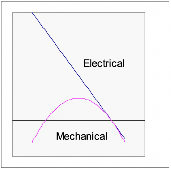Figure 4: DC Machine Operating Regimes

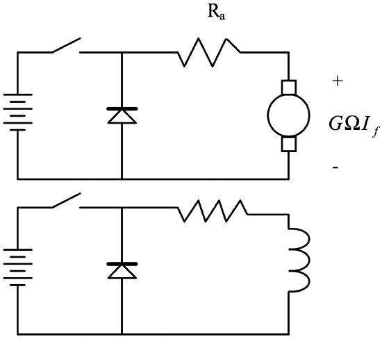Figure 5: Two-Chopper, separately excited machine hookup

some traction applications apply voltage control in the form of “choppers” to separately excited machines.

Note that the “zero torque speed” is dependend on armature voltage and on field current. For high torque at low speed one would operate the machine with high field current and enough armature voltage to produce the requisite current. As speed increases so does back voltage, and field current may need to be reduced. At any steady operating speed there will be some optimum mix of field and armature currents to produced the required torque. For braking one could (and this is often done) re-connect the armature of the machine to a braking resistor and turn the machine into a generator. Braking torque is controlled by field current.

A subset of the separately excited machine is the shunt connection in which armature and field are supplied by the same source, in parallel. This connection is not widely used any more: it does not yield any meaningful ability to control speed and the simple applications to which is used to be used are mostly being handled by induction machines.

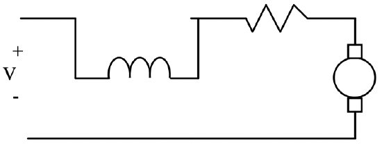Figure 6: Series Connection

Another connection which is still widely used in the series connection, in which the field winding is sized so that its normal operating current level is the same as normal armature current and the two windings are connected in series. Then:

\(\ I_{a}=I_{f}=\frac{V}{R_{a}+R_{f}+G \Omega}\)

And then torque is:

\(\ T_{e}=\frac{G V^{2}}{\left(R_{a}+R_{f}+G \Omega\right)^{2}}\)

It is important to note that this machine has no “zero-torque” speed, leading to the possibility that an unloaded machine might accelerate to dangerous speeds. This is particularly true because the commutator, made of pieces of relatively heavy material tied together with non- conductors, is not very strong.

Speed control of series connected machines can be achieved with voltage control and many appliances using this type of machine use choppers or phase control. An older form of control used in traction applications was the series dropping resistor: obviously not a very efficient way of controlling the machine and not widely used (except in old equipment, of course).

A variation on this class of machine is the very widely used “universal motor”, in which the stator and rotor (field and armature) of the machine are both constructed to operate with alternating current. This means that both the field and armature are made of laminated steel. Note that such a machine will operate just as it would have with direct current, with the only addition being the reactive impedance of the two windings. Working with RMS quantities:

\(\ \begin{aligned}
\underline{I} &=\frac{\underline{V}}{R_{a}+R_{f}+G \Omega+j \omega\left(L_{a}+L_{f}\right)} \\
T_{e} &=\frac{|\underline{V}|^{2}}{\left(R_{a}+R_{f}+G \Omega\right)^{2}+\left(\omega L_{a}+\omega L_{f}\right)^{2}}
\end{aligned}\)

where \(\ \omega\) is the electrical supply frequency. Note that, unlike other AC machines, the universal motor is not limited in speed to the supply frequency. Appliance motors typically turn substantially faster than the 3,600 RPM limit of AC motors, and this is one reason why they are so widely used: with the high rotational speeds it is possible to produce more power per unit mass (and more power per dollar).

Commutator

The commutator is what makes this machine work. The brush and commutator system of this class of motor involves quite a lot of “black art”, and there are still aspects of how they work which are poorly understood. However, we can make some attempt to show a bit of what the brush/commutator system does.

To start, take a look at the picture shown in Figure 7. Represented are a pair of poles (shaded) and a pair of brushes. Conductors make a group of closed paths. Current from one of the brushes takes two parallel paths. You can follow one of those paths around a closed loop, under each of the two poles (remember that the poles are of opposite polarity) to the opposite brush. Open commutator segments (most of them) do not carry current into or out of the machine.

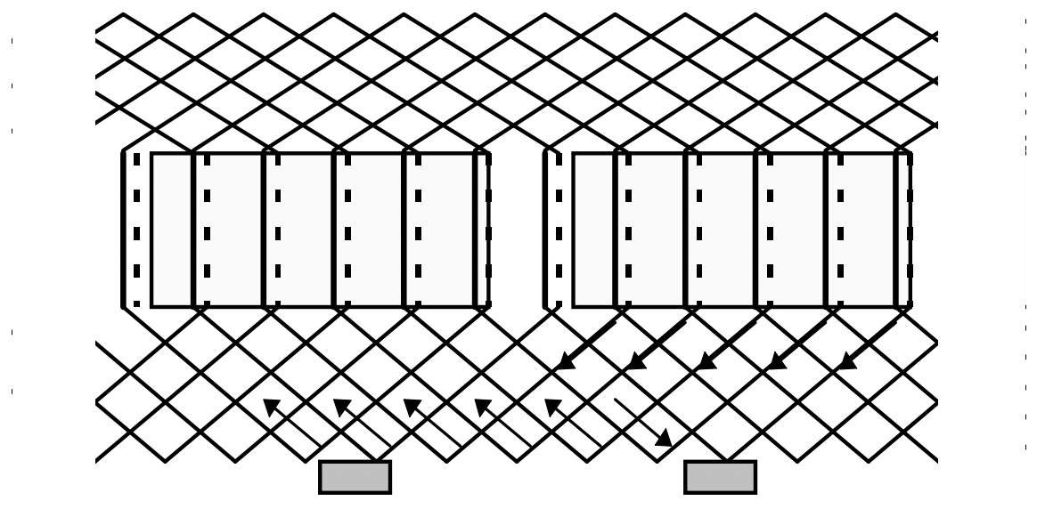Figure 7: Commutator and Current Paths

A commutation interval occurs when the current in one coil must be reversed. (See Figure 8 In the simplest form this involves a brush bridging between two commutator segments, shorting out that coil. The resistance of the brush causes the current to decay. When the brush leaves the leading segment the current in the leading coil must reverse.

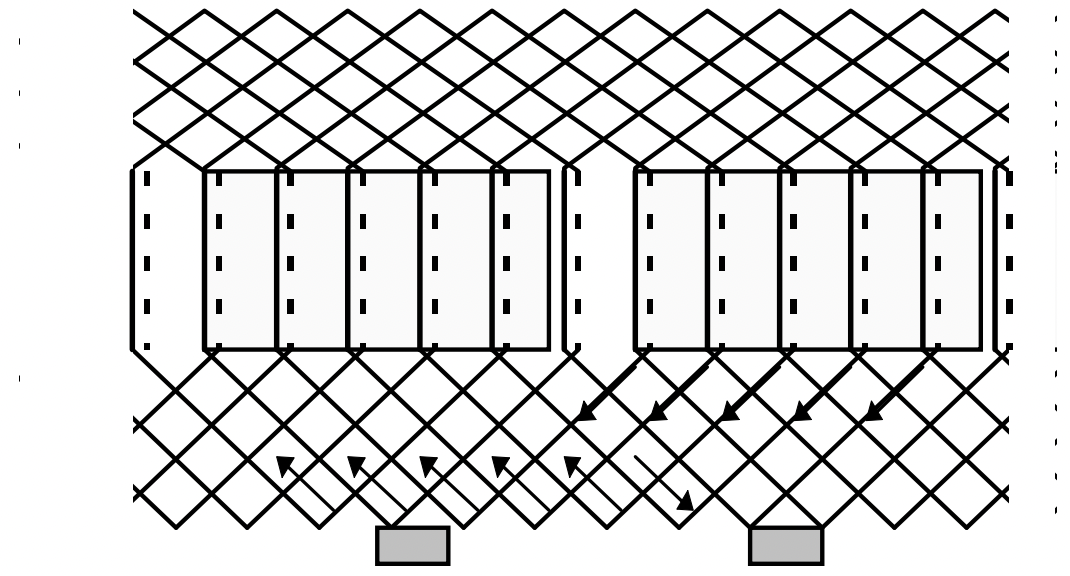Figure 8: Commutator at Commutation

We will not attempt to fully understand the commutation process in this type of machine, but we can note a few things. Resistive commutation is the process relied upon in small machines.

When the current in one coil must be reversed (because it has left one pole and is approaching the other), that coil is shorted by one of the brushes. The brush resistance causes the current in the coil to decay. Then the leading commutator segment leaves the brush the current MUST reverse (the trailing coil has current in it), and there is often sparking.

Commutation

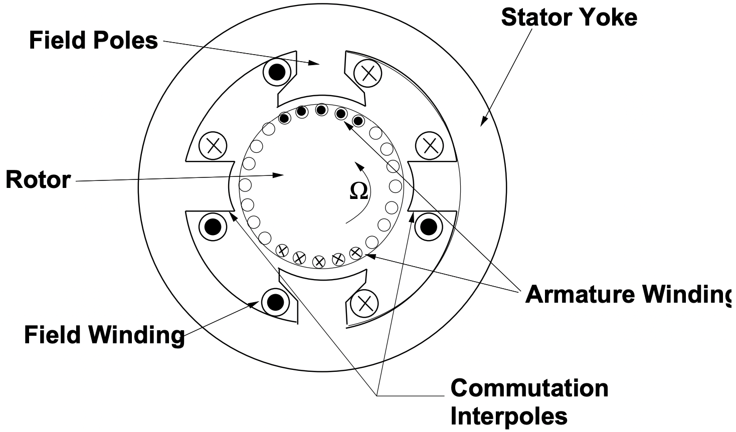Figure 9: Commutation Interpoles

In larger machines the commutation process would involve too much sparking, which causes brush wear, noxious gases (ozone) that promote corrosion, etc. In these cases it is common to use separate commutation interpoles. These are separate, usually narrow or seemingly vestigal pole pieces which carry armature current. They are arranged in such a way that the flux from the interpole drives current in the commutated coil in the proper direction. Remember that the coil being commutated is located physically between the active poles and the interpole is therefore in the right spot to influence commutation. The interpole is wound with armature current (it is in series with the main brushes). It is easy to see that the interpole must have a flux density proportional to the current to be commutated. Since the speed with which the coil must be commutated is proportional to rotational velocity and so is the voltage induced by the interpole, if the right number of turns are put around the interpole, commutation can be made to be quite accurate.

Compensation

The analysis of commutator machines often ignores armature reaction flux. Obviously these machines DO produce armature reaction flux, in quadrature with the main field. Normally, commutator machines are highly salient and the quadrature inductance is lower than direct-axis inductance, but there is still flux produced. This adds to the flux density on one side of the main poles (possibly leading to saturation). To make the flux distribution more uniform and therefore to avoid this saturation effect of quadrature axis flux, it is common in very highly rated machines to wind compensation coils: essentially mirror-images of the armature coils, but this time wound in slots in the surface of the field poles. Such coils will have the same number of ampere-turns as the

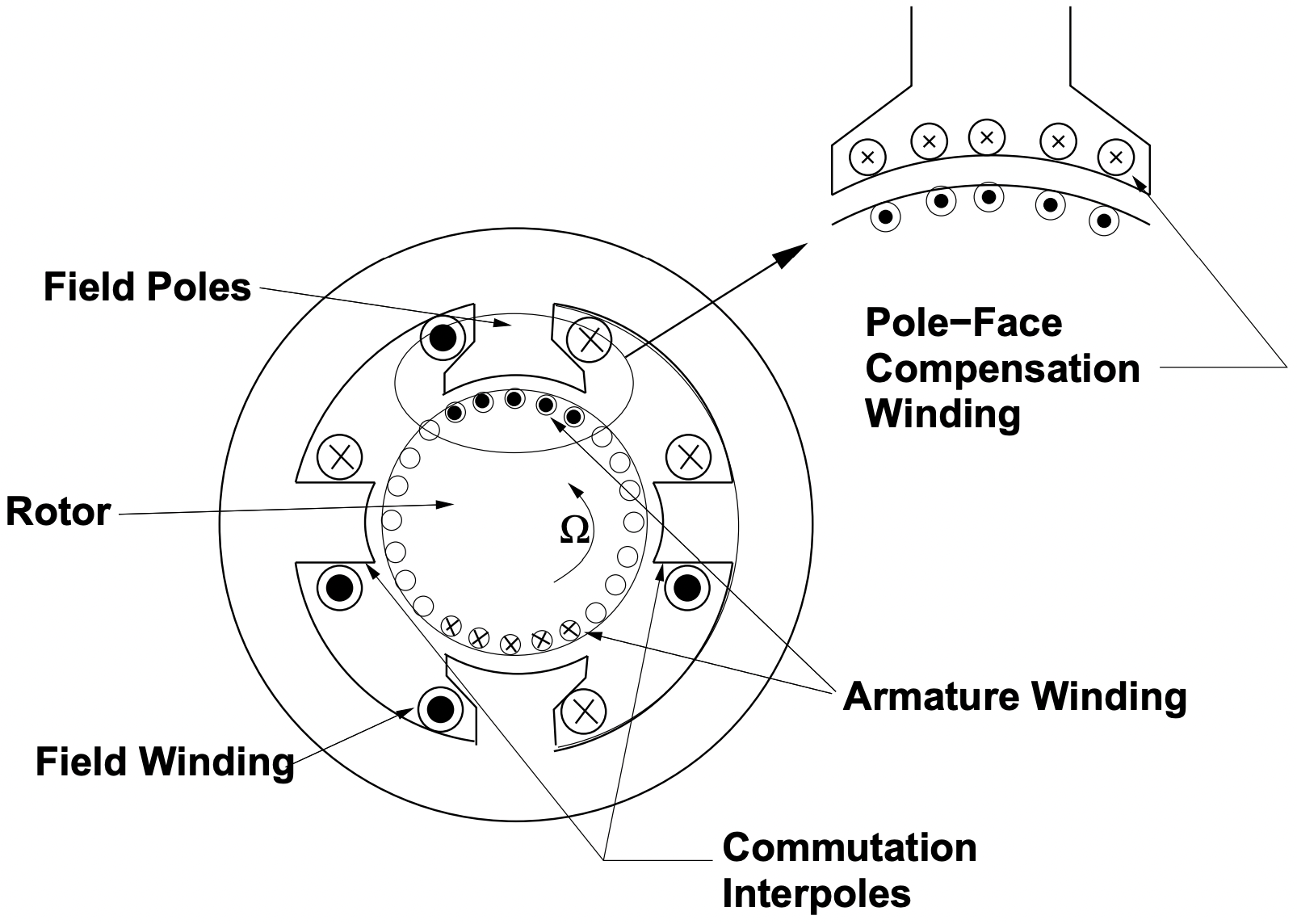Figure 10: Pole Face Compensation Winding

armature. Normally they have the same number of turns and are connected directly in series with the armature brushes. What they do is to almost exactly cancel the flux produced by the armature coils, leaving only the main flux produced by the field winding. One might think of these coils as providing a reaction torque, produced in exactly the same way as main torque is produced by the armature. A cartoon view of this is shown in Figure 10.