11.2: Permanent Magnets in Electric Machines

Of all changes in materials technology over the last several years, advances in permanent magnets have had the largest impact on electric machines. Permanent magnets are often suitable as replacements for the field windings in machines: that is they can produce the fundamental interaction field. This does three things. First, since the permanent magnet is lossless it eliminates the energy required for excitation, usually improving the efficiency of the machine. Second, since eliminating the excitation loss reduces the heat load it is often possible to make PM machines more compact. Finally, and less appreciated, is the fact that modern permanent magnets have very large coercive force densities which permit vastly larger air gaps than conventional field windings, and this in turn permits design flexibility which can result in even better electric machines.

These advantages come not without cost. Permanent magnet materials have special characteristics which must be taken into account in machine design. The highest performance permanent magnets are brittle ceramics, some have chemical sensitivities, all are sensitive to high temperatures, most have sensitivity to demagnetizing fields, and proper machine design requires understanding the materials well. These notes will not make you into seasoned permanent magnet machine designers. They are, however, an attempt to get started, to develop some of the mathematical skills required and to point to some of the important issues involved.

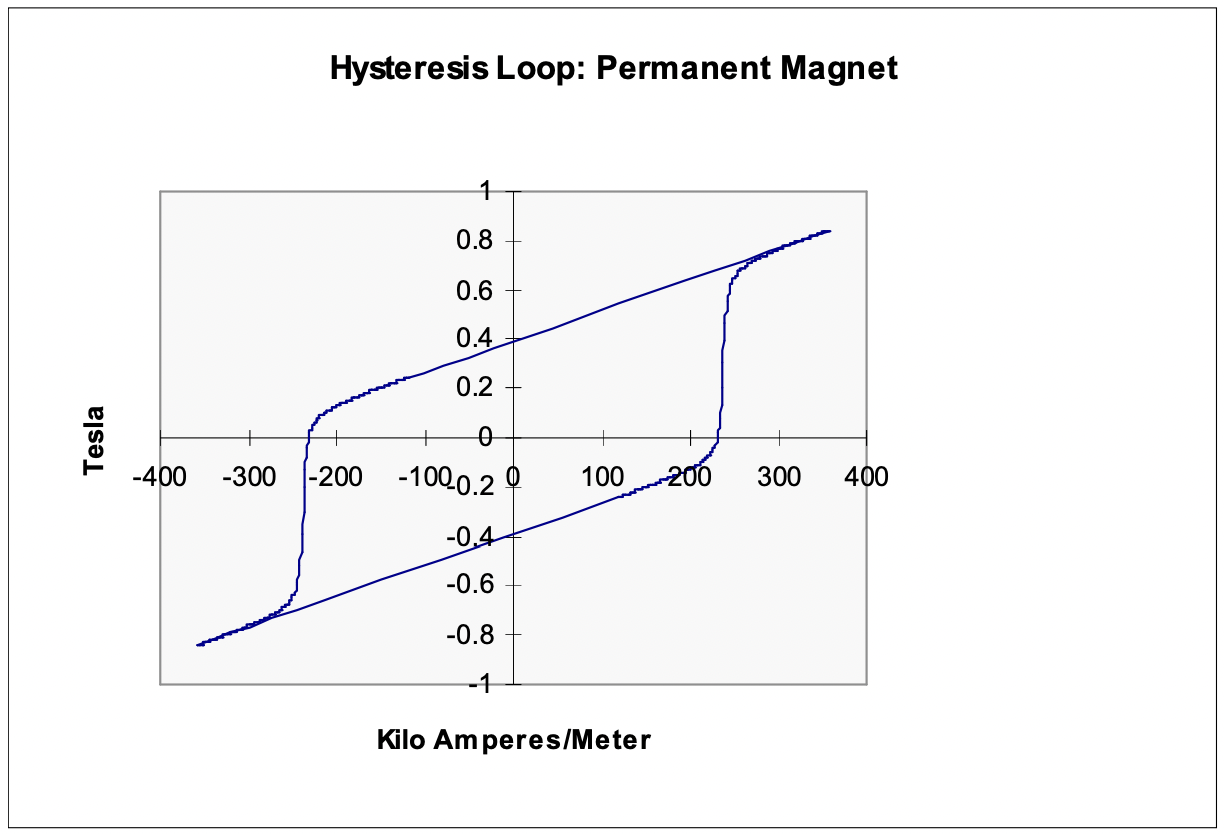Figure 11: Hysteresis Loop Of Ceramic Permanent Magnet

Permanent magnet materials are, at core, just materials with very wide hysteresis loops. Figure 11 is an example of something close to one of the more popular ceramic magnet materials.Note that this hysteresis loop is so wide that you can see the effect of the permeability of free space.

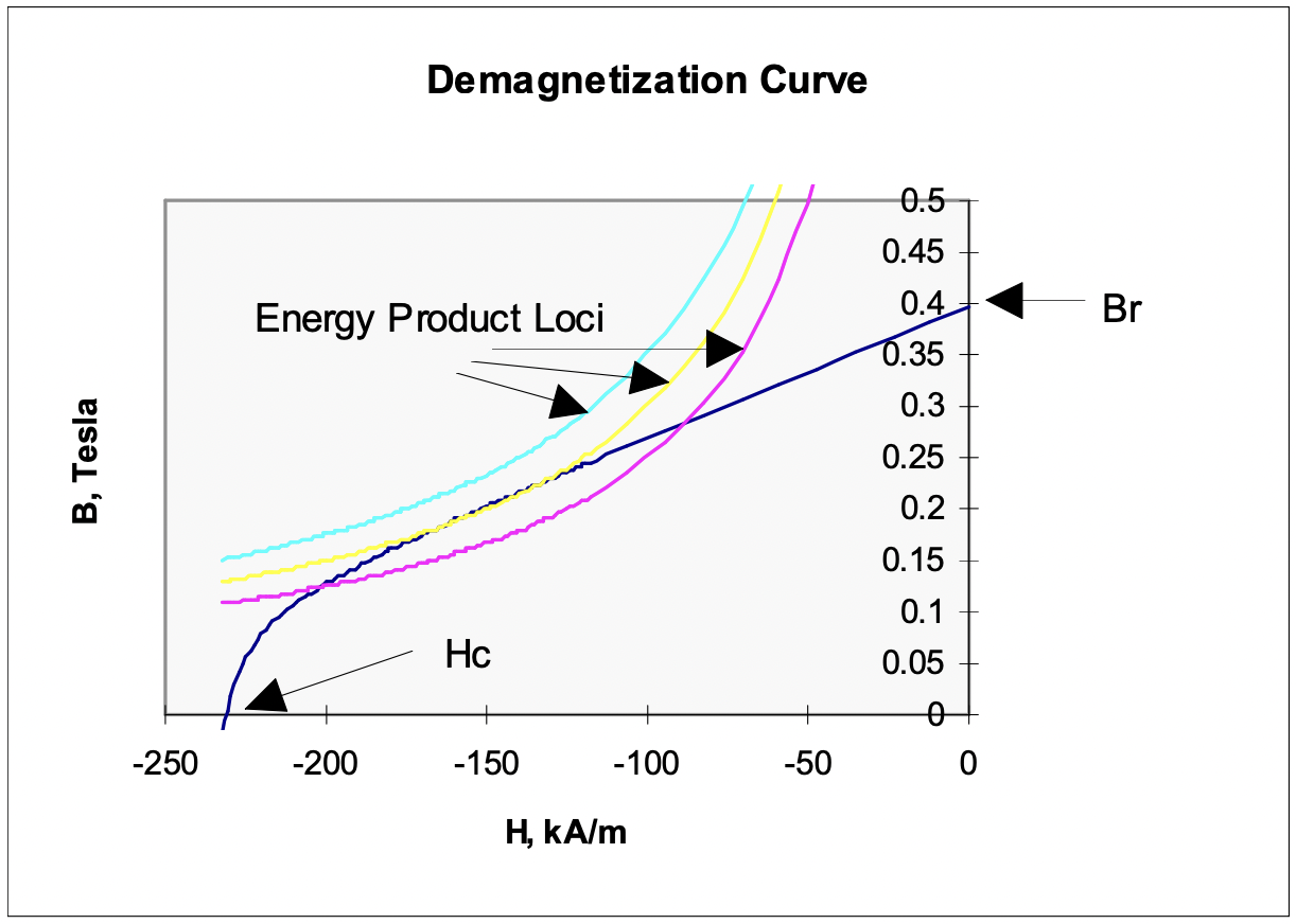Figure 12: Demagnetization Curve

It is usual to display only part of the magnetic characteristic of permanent magnet materials (see Figure 12), the third quadrant of this picture, because that is where the material is normally operated. Note a few important characteristics of what is called the “demagnetization curve”. The remanent flux density \(\ B_{r}\), is the value of flux density in the material with zero magnetic field \(\ H\). The coercive field \(\ H_{c}\) is the magnetic field at which the flux density falls to zero. Shown also on the curve are loci of constant energy product. This quantity is unfortunately named, for although it has the same units as energy it represents real energy in only a fairly general sense. It is the product of flux density and field intensity. As you already know, there are three commonly used systems of units for magnetic field quantities, and these systems are often mixed up to form very confusing units. We will try to stay away from the English system of units in which field intensity \(\ H\) is measured in amperes per inch and flux density \(\ B\) in lines (actually, usually kilolines) per square inch. In CGS units flux density is measured in Gauss (or kilogauss) and magnetic field intensity in Oersteds. And in SI the unit of flux density is the Tesla, which is one Weber per square meter, and the unit of field intensity is the Ampere per meter. Of these, only the last one, \(\ A / m\) is obvious. A Weber is a vo }\) Tesla. And, finally, an Oersted is that field intensity required to produce one Gauss in the permeability of free space. Since the permeability of free space \(\ \mu_{0}=4 \pi \times 10^{-7} H y / m\), this means that one Oe is about 79.58 A/m. Commonly, the energy product is cited in MgOe (Mega-Gauss-Oersted)s. One MgOe is equal to \(\ 7.958 k \mathrm{~J} / \mathrm{m}^{3}\). A commonly used measure for the performance of a permanent magnet material is the maximum energy product, the largest value of this product along the demagnetization curve.

To start to understand how these materials might be useful, consider the situation shown in Figure 13: A piece of permanent magnet material is wrapped in a magnetic circuit with effectively infinite permeability. Assume the thing has some (finite) depth in the direction you can’t see. Now, if we take Ampere’s law around the path described by the dotted line,

\(\ \oint \vec{H} \cdot d \vec{\ell}=0\)

since there is no current anywhere in the problem. If magnetization is upwards, as indicated by the arrow, this would indicate that the flux density in the permanent magnet material is equal to the remanent flux density (also upward).

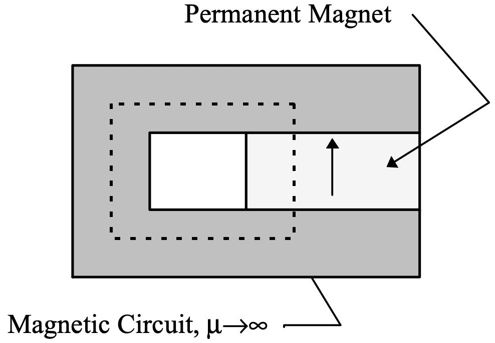Figure 13: Permanent Magnet in Magnetic Circuit

A second problem is illustrated in Figure 14, in which the same magnet is embedded in a magnetic circuit with an air gap. Assume that the gap has width g and area Ag. The magnet has height hm and area Am. For convenience, we will take the positive reference direction to be up (as we see it here) in the magnet and down in the air-gap.

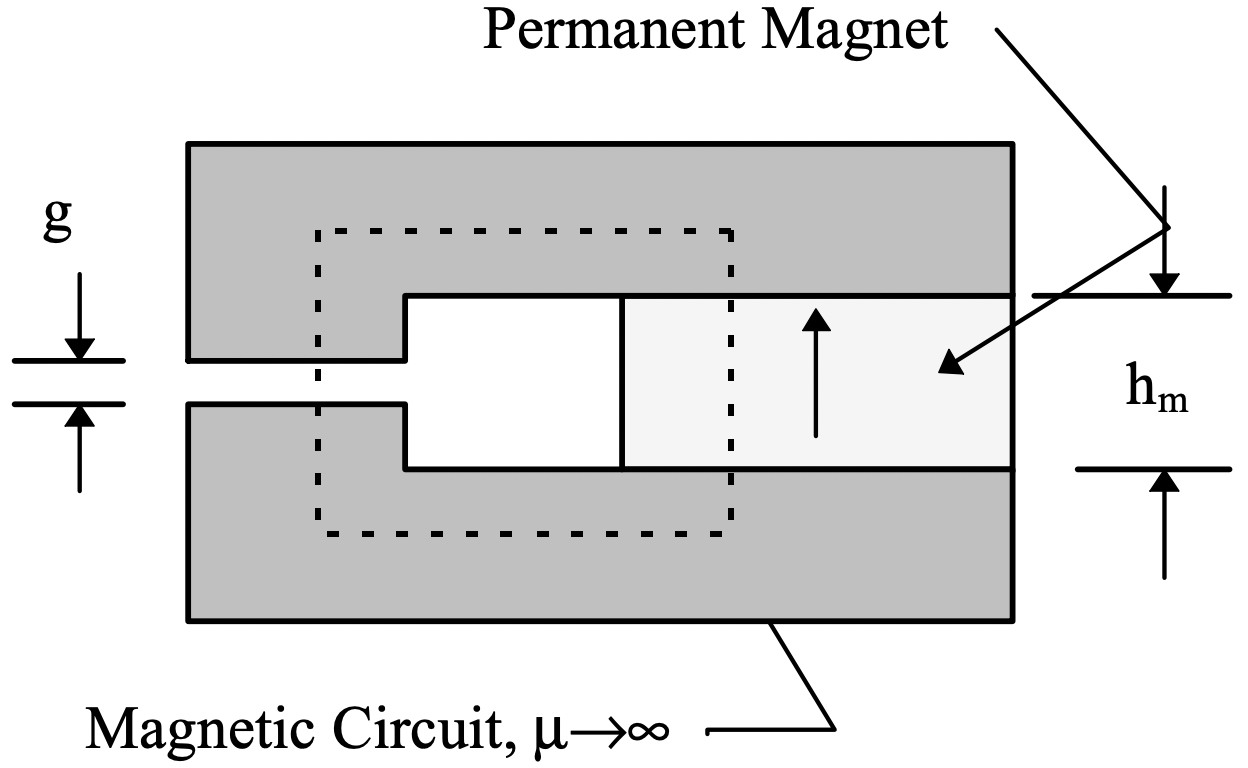Figure 14: Permanent Magnet Driving an Air-Gap

Thus we are following the same reference direction as we go around the Ampere’s Law loop. That becomes:

\(\ \oint \vec{H} \cdot d \vec{\ell}=H_{m} h_{m}+H_{g} g\)

Now, Gauss’ law could be written for either the upper or lower piece of the magnetic circuit. Assuming that the only substantive flux leaving or entering the magnetic circuit is either in the magnet or the gap:

\(\ \oiint \vec{B} \cdot d \vec{A}=B_{m} A_{m}-\mu_{0} H_{g} A_{g}\)

Solving this pair we have:

\(\ B_{m}=-\mu_{0} \frac{A_{g}}{A_{m}} \frac{h_{m}}{g} H_{m}=\mu_{0} \mathcal{P}_{u} H_{m}\)

This defines the unit permeance, essentially the ratio of the permeance facing the permanent magnet to the internal permeance of the magnet. The problem can be, if necessary, solved graphically, since the relationship between \(\ B_{m}\) and \(\ H_{m}\) is inherently nonlinear, as shown in Figure 15 “load line” analysis of a nonlinear electronic circuit.

Now, one more ‘cut’ at this problem. Note that, at least for fairly large unit permeances the slope of the magnet characteristic is fairly constant. In fact, for most of the permanent magnets used in machines (the one important exception is the now rarely used ALNICO alloy magnet), it is generally acceptable to approximate the demagnitization curve with:

\(\ \vec{B}_{m}=\mu_{m}\left(\vec{H}_{m}+\vec{M}_{0}\right)\)

Here, the magnetization \(\ M_{0}\) is fixed. Further, for almost all of the practical magnet materials the magnet permeability is nearly the same as that of free space \(\ \left(\mu_{m} \approx \mu_{0}\right)\). With that in mind,

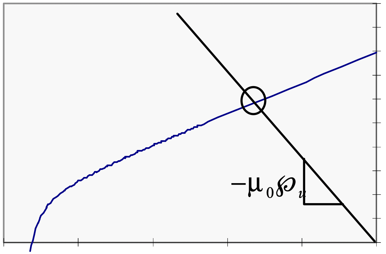Figure 15: Load Line, Unit Permeance Analysis

consider the problem shown in Figure 16, in which the magnet fills only part of a gap in a magnetic circuit. But here the magnet and gap areas are essentially the same. We could regard the magnet as simply a magnetization.

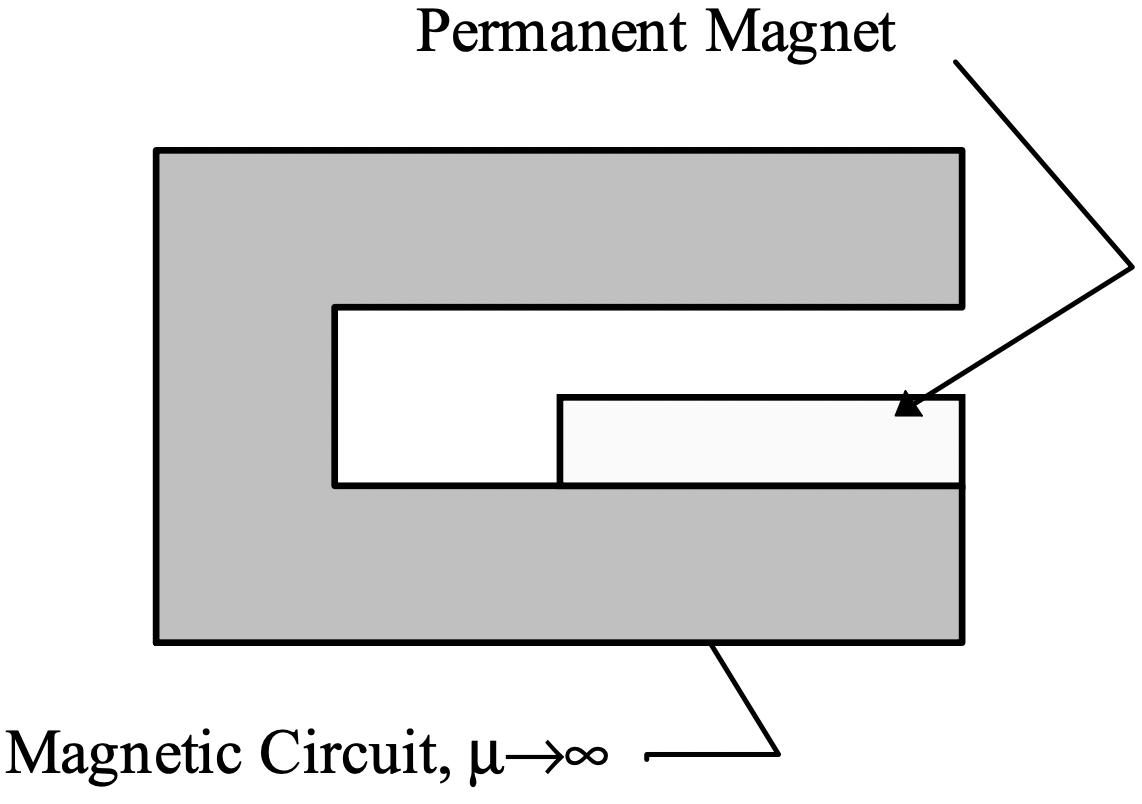Figure 16: Surface Magnet Primitive Problem

In the region of the magnet and the air-gap, Ampere’s Law and Gauss’ law can be written:

\(\ \begin{aligned}
\nabla \times \vec{H} &=0 \\
\nabla \cdot \mu_{0}\left(\vec{H}_{m}+\vec{M}_{0}\right) &=0 \\
\nabla \cdot \mu_{0} \vec{H}_{g} &=0
\end{aligned}\)

Now, if in the magnet the magnetization is constant, the divergence of \(\ H\) in the magnet is zero. Because there is no current here, \(\ H\) is curl free, so that everywhere:

\(\ \begin{aligned}
\vec{H} &=-\nabla \psi \\
\nabla^{2} \psi &=0
\end{aligned}\)

That is, magnetic field can be expressed as the gradient of a scalar potential which satisfies Laplace’s equation. It is also pretty clear that, if we can assign the scalar potential to have a value of zero anywhere on the surface of the magnetic circuit it will be zero over all of the magnetic circuit (i.e. at both the top of the gap and the bottom of the magnet). Finally, note that we can’t actually assume that the scalar potential satisfies Laplace’s equation everywhere in the problem. In fact the divergence of M is zero everywhere except at the top surface of the magnet where it is singular! In fact, we can note that there is a (some would say fictitious) magnetic charge density:

\(\ \rho_{m}=-\nabla \cdot \vec{M}\)

At the top of the magnet there is a discontinuous change in M and so the equivalent of a magnetic surface charge. Using \(\ H_{g}\) to note the magnetic field above the magnet and \(\ H_{m}\) to note the magnetic field in the magnet,

\(\ \begin{aligned}
\mu_{0} H_{g} &=\mu_{0}\left(H_{m}+M_{0}\right) \\
\sigma_{m} &=M_{0}=H_{g}-H_{m}
\end{aligned}\)

and then to satisfy the potential condition, if hm is the height of the magnet and g is the gap:

\(\ g H_{g}=h_{m} H_{m}\)

Solving,

\(\ H_{g}=M_{0} \frac{h_{m}}{h_{m}+g}\)

Now, one more observation could be made. We would produce the same air-gap flux density if we regard the permanent magnet as having a surface current around the periphery equal to the magnetization intensity. That is, if the surface current runs around the magnet:

\(\ K_{\phi}=M_{0}\)

This would produce an MMF in the gap of:

\(\ F=K_{\phi} h_{m}\)

and then since the magnetic field is just the MMF divided by the total gap:

\(\ H_{g}=\frac{F}{h_{m}+g}=M_{0} \frac{h_{m}}{h_{m}+g}\)

The real utility of permanent magnets comes about from the relatively large magnetizations: numbers of a few to several thousand amperes per meter are common, and these would translate into enormous current densities in magnets of ordinary size.