11.3: Simple Permanent Magnet Machine Structures- Commutator Machines

Figure 17 is a cartoon picture of a cross section of the geometry of a two-pole commutator machine using permanent magnets. This is actually the most common geometry that is used. The rotor (armature) of the machine is a conventional, windings-in-slots type, just as we have already seen

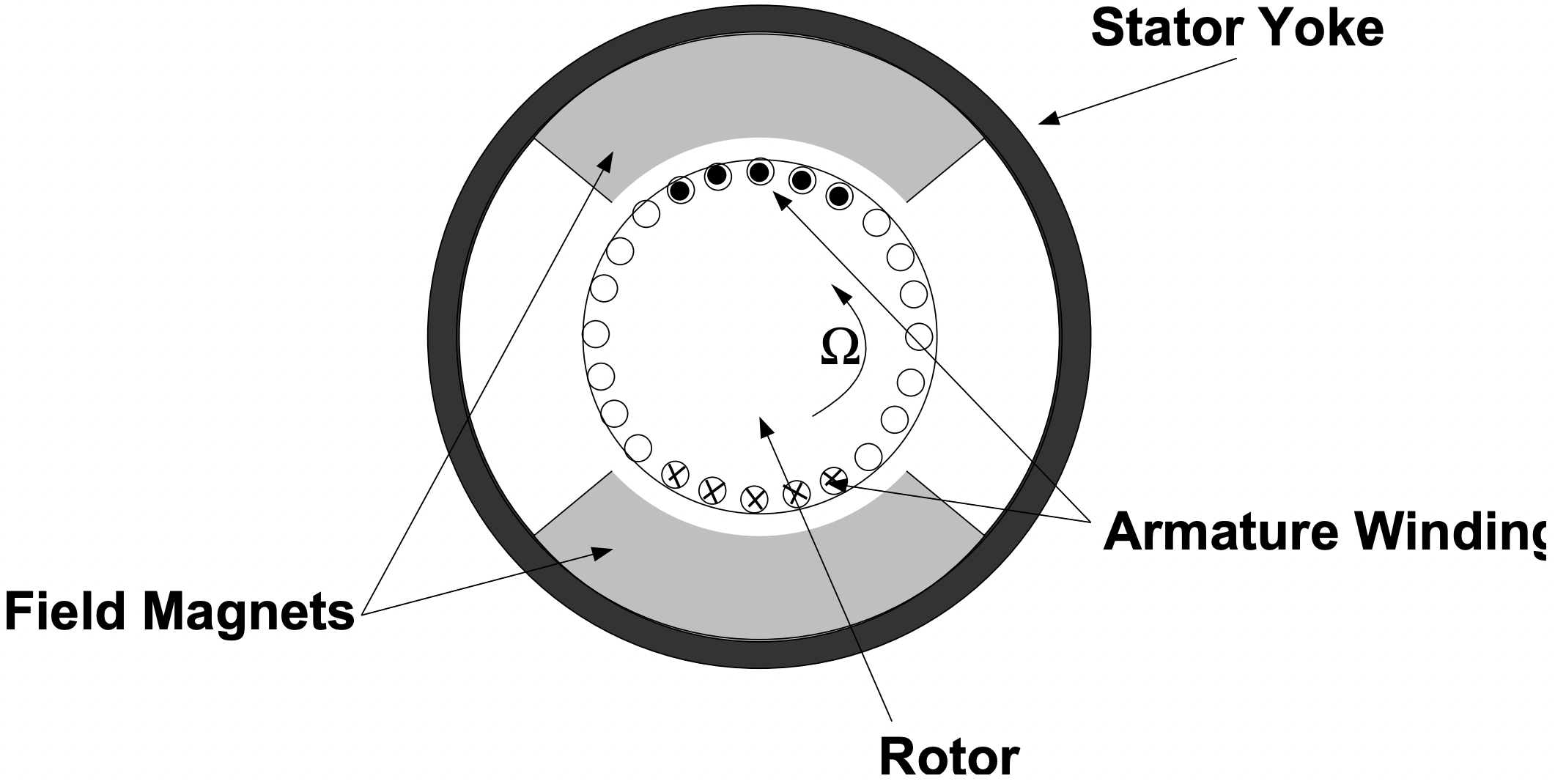Figure 17: PM Commutator Machine

for commutator machines. The field magnets are fastened (often just bonded) to the inside of a steel tube that serves as the magnetic flux return path.

Assume for the purpose of first-order analysis of this thing that the magnet is describable by its remanent flux density \(\ B_{r}\) and had permeability of \(\ \mu_{0}\). First, we will estimate the useful magnetic flux density and then will deal with voltage generated in the armature. Interaction Flux Density Using the basics of the analysis presented above, we may estimate the radial magnetic flux density at the air-gap as being:

\(\ B_{d}=\frac{B_{r}}{1+\frac{1}{\mathcal{P}_{c}}}\)

where the effective unit permeance is:

\(\ \mathcal{P}_{c}=\frac{f_{l}}{f_{f}} \frac{h_{m}}{g} \frac{A_{g}}{A_{m}}\)

A book on this topic by James Ireland suggests values for the two “fudge factors”:

1. The “leakage factor” \(\ f_{l}\) is cited as being about 1.1.
2. The “reluctance factor” \(\ f_{f}\) is cites as being about 1.2.

We may further estimate the ratio of areas of the gap and magnet by:

\(\ \frac{A_{g}}{A_{m}}=\frac{R+\frac{g}{2}}{R+g+\frac{h_{m}}{2}}\)

Now, there are a bunch of approximations and hand wavings in this expression, but it seems to work, at least for the kind of machines contemplated.

A second correction is required to correct the effective length for electrical interaction. The reason for this is that the magnets produce fringing fields, as if they were longer than the actual ”stack length” of the rotor (sometimes they actually are). This is purely empirical, and Ireland gives a value for effective length for voltage generation of:

\(\ \ell_{\mathrm{eff}}=\frac{\ell^{*}}{f_{\ell}}\)

where \(\ \ell^{*}=\ell+2 N R\), and the empirical coefficient

\(\ N \approx \frac{A}{B} \log \left(1+B \frac{h_{m}}{R}\right)\)

where

\(\ \begin{aligned}
B &=7.4-9.0 \frac{h_{m}}{R} \\
A &=0.9
\end{aligned}\)

Voltage

It is, in this case, simplest to consider voltage generated in a single wire first. If the machine is running at angular velocity Ω, speed voltage is, while the wire is under a magnet,

\(\ v_{s}=\Omega R \ell B_{r}\)

Now, if the magnets have angular extent \(\ \theta_{m}\) the voltage induced in a wire will have a waveform as shown in Figure 18: It is pulse-like and has the same shape as the magnetic field of the magnets.

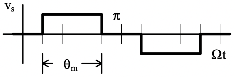Figure 18: Voltage Induced in One Conductor

The voltage produced by a coil is actually made up of two waveforms of exactly this form, but separated in time by the ”coil throw” angle. Then the total voltage waveform produced will be the sum of the two waveforms. If the coil thrown angle is larger than the magnet angle, the two voltage waveforms add to look like this: There are actually two coil-side waveforms that add with a slight phase shift.

If, on the other hand, the coil thrown is smaller than the magnet angle, the picture is the same, only the width of the pulses is that of the coil rather than the magnet. In either case the average voltage generated by a coil is:

\(\ v=\Omega R \ell N_{s} \frac{\theta^{*}}{\pi} B_{d}\)

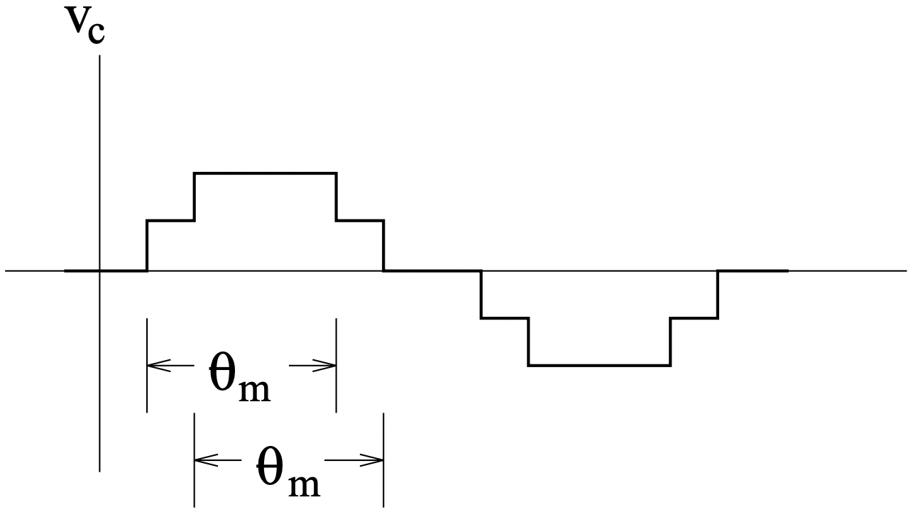Figure 19: Voltage Induced in a Coil

where \(\ \theta^{*}\) is the lesser of the coil throw or magnet angles and \(\ N_{s}\) is the number of series turns in the coil. This gives us the opportunity to develop the number of “active” turns:

\(\ \frac{C_{a}}{m}=N_{s} \frac{\theta^{*}}{\pi}=\frac{C_{\mathrm{tot}}}{m} \frac{\theta^{*}}{\pi}\)

Here, \(\ C_{a}\) is the number of active conductors, \(\ C_{\text {tot }}\) is the total number of conductors and \(\ m\) is the number of parallel paths. The motor coefficient is then:

\(\ K=\frac{R \ell_{\mathrm{eff}} C_{\mathrm{tot}} B_{d}}{m} \frac{\theta^{*}}{\pi}\)

Armature Resistance

The last element we need for first-order prediction of performance of the motor is the value of armature resistance. The armature resistance is simply determined by the length and area of the wire and by the number of parallel paths (generally equal to 2 for small commutator motors). If we note \(\ N_{c}\) as the number of coils and \(\ N_{a}\) as the number of turns per coil,

\(\ N_{s}=\frac{N_{c} N_{a}}{m}\)

Total armature resistance is given by:

\(\ R_{a}=2 \rho_{w} \ell_{t} \frac{N_{s}}{m}\)

where \(\ \rho_{w}\) is the resistivity (per unit length) of the wire:

\(\ \rho_{w}=\frac{1}{\frac{\pi}{4} d_{w}^{2} \sigma_{w}}\)

(\(\ d_{w}\) is wire diameter, \(\ \sigma_{w}\) is wire conductivity and \(\ \ell_{t}\) is length of one half-turn). This length depends on how the machine is wound, but a good first-order guess might be something like this:

\(\ \ell_{t} \approx \ell+\pi R\)