12.2: Zeroth Order Rating

In determining the rating of a machine, we may consider two separate sets of parameters. The first set, the elementary rating parameters, consist of the machine inductances, internal flux linkage and stator resistance. From these and a few assumptions about base and maximum speed it is possible to get a first estimate of the rating and performance of the motor. More detailed performance estimates, including efficiency in sustained operation, require estimation of other parameters. We will pay more attention to that first set of parameters, but will attempt to show how at least some of the more complete operating parameters can be estimated.

Voltage and Current: Round Rotor

To get started, consider the equivalent circuit shown in Figure 5. This is actually the equivalent circuit which describes all round rotor synchronous machines. It is directly equivalent only to some of the machines we are dealing with here, but it will serve to illustrate one or two important points.

What is shown here is the equivalent circuit of a single phase of the machine. Most motors are three-phase, but it is not difficult to carry out most of the analysis for an arbitrary number of phases. The circuit shows an internal voltage \(\ E_{a}\) and a reactance \(\ X\) which together with the terminal current \(\ I\) determine the terminal voltage \(\ V\). In this picture armature resistance is ignored. If the machine is running in the sinusoidal steady state, the major quantities are of the form:

\(\ \begin{aligned}
E_{a} &=\omega \lambda_{a} \cos (\omega t+\delta) \\
V_{t} &=V \cos \omega t \\
I_{a} &=I \cos (\omega t-\psi)
\end{aligned}\)

The machine is in synchronous operation if the internal and external voltages are at the same

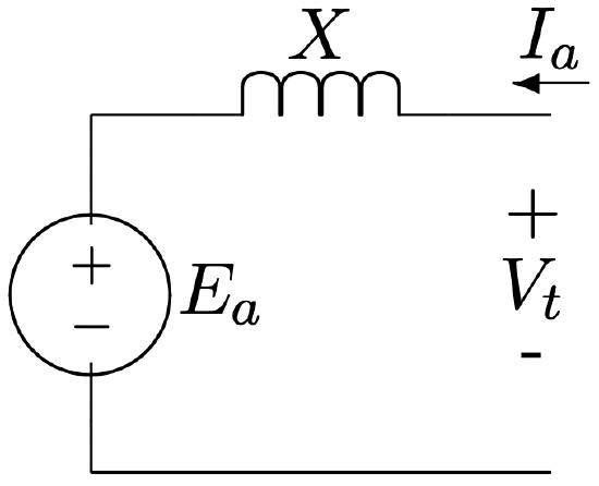Figure 5: Synchronous Machine Equivalent Circuit

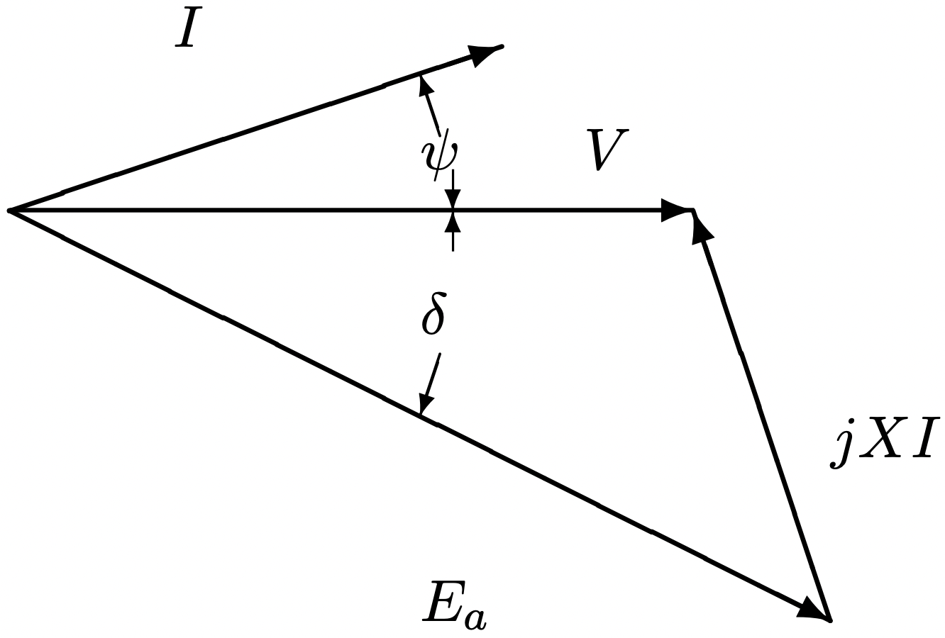Figure 6: Phasor Diagram For A Synchronous Machine

frequency and have a constant (or slowly changing) phase relationship \(\ (\delta)\). The relationship between the major variables may be visualized by the phasor diagram shown in Figure 3.1. The internal voltage is just the time derivative of the internal flux from the permanent magnets, and the voltage drop in the machine reactance is also the time derivative of flux produced by armature current in the air-gap and in the “leakage” inductances of the machine. By convention, the angle \(\ \psi\) is positive when current \(\ I\) lags voltage \(\ V\) and the angle \(\ \delta\) is positive then internal voltage \(\ E_{a}\) leads terminal voltage \(\ V\). So both of these angles have negative sign in the situation shown in Figure 3.1.

If there are \(\ q\) phases, the time average power produced by this machine is simply:

\(\ P=\frac{q}{2} V I \cos \psi\)

For most polyphase machines operating in what is called “balanced” operation (all phases doing the same thing with uniform phase differences between phases), torque (and consequently power) are approximately constant. Since we have ignored power dissipated in the machine armature, it must be true that power absorbed by the internal voltage source is the same as terminal power, or:

\(\ P=\frac{q}{2} E_{a} I \cos (\psi-\delta)\)

Since in the steady state:

\(\ P=\frac{\omega}{p} T\)

where \(\ T\) is torque and \(\ \omega / p\) is mechanical rotational speed, torque can be derived from the terminal quantities by simply:

\(\ T=p \frac{q}{2} \lambda_{a} I \cos (\psi-\delta)\)

In principal, then, to determine the torque and hence power rating of a machine it is only necessary to determine the internal flux, the terminal current capability, and the speed capability of the rotor. In fact it is almost that simple. Unfortunately, the model shown in Figure 5 is not quite complete for some of the motors we will be dealing with, and we must go one more level into machine theory.

A Little Two-Reaction Theory

The material in this subsection is framed in terms of three-phase \(\ (q=3)\) machine theory, but it is actually generalizable to an arbitrary number of phases. Suppose we have a machine whose three-phase armature can be characterized by internal fluxes and inductance which may, in general, not be constant but is a function of rotor position. Note that the simple model we presented in the previous subsection does not conform to this picture, because it assumes a constant terminal inductance. In that case, we have:

\[\ \underline{\lambda}_{p h}=\underline{\underline{L}}_{p h} \underline{\underline{I}}_{p h}+\underline{\lambda_{R}}\label{1} \]

where \(\ \underline{\lambda_{R}}\) is the set of internally produced fluxes (from the permanent magnets) and the stator winding may have both self- and mutual- inductances.

Now, we find it useful to do a transformation on these stator fluxes in the following way: each armature quantity, including flux, current and voltage, is projected into a coordinate system that is fixed to the rotor. This is often called the Park’s Transformation. For a three phase machine it is:

\[\ \left[\begin{array}{c}
u_{d} \\
u_{q} \\
u_{0}
\end{array}\right]=\underline{u}_{d q}=\underline{\underline{T}u} _{p h}=\underline{\underline{T}}\left[\begin{array}{l}
u_{a} \\
u_{b} \\
u_{c}
\end{array}\right]\label{2} \]

Where the transformation and its inverse are:

\[\ \underline{\underline{T}}=\frac{2}{3}\left[\begin{array}{ccc}
\cos \theta & \cos \left(\theta-\frac{2 \pi}{3}\right) & \cos \left(\theta+\frac{2 \pi}{3}\right) \\
-\sin \theta & -\sin \left(\theta-\frac{2 \pi}{3}\right) & -\sin \left(\theta+\frac{2 \pi}{3}\right) \\
\frac{1}{2} & \frac{1}{2} & \frac{1}{2}
\end{array}\right]\label{3} \]

\[\ \underline{\underline{T}}^{-1}=\left[\begin{array}{ccc}
\cos \theta & -\sin \theta & 1 \\
\cos \left(\theta-\frac{2 \pi}{3}\right) & -\sin \left(\theta-\frac{2 \pi}{3}\right) & 1 \\
\cos \left(\theta+\frac{2 \pi}{3}\right) & -\sin \left(\theta+\frac{2 \pi}{3}\right) & 1
\end{array}\right]\label{4} \]

It is easy to show that balanced polyphase quantities in the stationary, or phase variable frame, translate into constant quantities in the so-called “d-q” frame. For example:

\(\ \begin{aligned}
I_{a} &=I \cos \omega t \\
I_{b} &=I \cos \left(\omega t-\frac{2 \pi}{3}\right) \\
I_{c} &=I \cos \left(\omega t+\frac{2 \pi}{3}\right) \\
\theta &=\omega t+\theta_{0}
\end{aligned}\)

maps to:

\(\ \begin{aligned}
I_{d} &=I \cos \theta_{0} \\
I_{q} &=-I \sin \theta_{0}
\end{aligned}\)

Now, if \(\ \theta=\omega t+\theta_{0}\), the transformation coordinate system is chosen correctly and the “d-” axis will correspond with the axis on which the rotor magnets are making positive flux. That happens if, when \(\ \theta=0\), phase A is linking maximum positive flux from the permanent magnets. If this is the case, the internal fluxes are:

\(\ \begin{array}{l}
\lambda_{a a}=\lambda_{f} \cos \theta \\
\lambda_{a b}=\lambda_{f} \cos \left(\theta-\frac{2 \pi}{3}\right) \\
\lambda_{a c}=\lambda_{f} \cos \left(\theta+\frac{2 \pi}{3}\right)
\end{array}\)

Now, if we compute the fluxes in the d-q frame, we have:

\[\ \underline{\lambda}_{d q}=\underline{\underline{L}}_{d q} \underline{I}_{d q}+\underline{\lambda}_{R}=\underline{\underline{T L}}_ {p h} \underline{\underline{T}}^{-1} \underline{I}_{d q}+\underline{\lambda}_{R}\label{5} \]

Now: two things should be noted here. The first is that, if the coordinate system has been chosen as described above, the flux induced by the rotor is, in the d-q frame, simply:

\[\ \underline{\lambda}_{R}=\left[\begin{array}{l}
\lambda_{f} \\
0 \\
0
\end{array}\right]\label{6} \]

That is, the magnets produce flux only on the d- axis.

The second thing to note is that, under certain assumptions, the inductances in the d-q frame are independent of rotor position and have no mutual terms. That is:

\[\ \underline{\underline{L}}_{d q}=\underline{\underline{T L}}_{p h} \underline{\underline{T}}^{-1}=\left[\begin{array}{lll}
L_{d} & 0 & 0 \\
0 & L_{q} & 0 \\
0 & 0 & L_{0}
\end{array}\right]\label{7} \]

The assertion that inductances in the d-q frame are constant is actually questionable, but it is close enough to being true and analyses that use it have proven to be close enough to being correct that it (the assertion) has held up to the test of time. In fact the deviations from independence on rotor position are small. Independence of axes (that is, absence of mutual inductances in the d-q frame) is correct because the two axes are physically orthogonal. We tend to ignore the third, or “zero” axis in this analysis. It doesn’t couple to anything else and has neither flux nor current anyway. Note that the direct- and quadrature- axis inductances are in principle straightforward to compute. They are

direct axis the inductance of one of the armature phases (corrected for the fact of multiple phases) with the rotor aligned with the axis of the phase, and

quadrature axis the inductance of one of the phases with the rotor aligned 90 electrical degrees away from the axis of that phase.

Next, armature voltage is, ignoring resistance, given by:

\[\ \underline{V}_{p h}=\frac{d}{d t} \underline{\lambda}_{p h}=\frac{d}{d t} \underline{\underline{T}}^{-1} \underline{\lambda}_{d q}\label{8} \]

and that the transformed armature voltage must be:

\[\ \begin{aligned}
\underline{V}_{d q} &=\underline{\underline{T }V}_{p h} \\
&=\underline{\underline{T}} \frac{d}{d t}\left(\underline{\underline{T}}^{-1} \underline{\lambda}_{d q}\right) \\
&=\frac{d}{d t} \underline{\lambda}_{d q}+\left(\underline{\underline{T}} \frac{d}{d t} \underline{\underline{T}}^{-1}\right) \underline{\lambda}_{d q}
\end{aligned}\label{9} \]

The second term in this expresses “speed voltage”. A good deal of straightforward but tedious manipulation yields:

\[\ \underline{\underline{T}} \frac{d}{d t} \underline{\underline{T}}^{-1}=\left[\begin{array}{ccc}
0 & -\frac{d \theta}{d t} & 0 \\
\frac{d \theta}{d t} & 0 & 0 \\
0 & 0 & 0
\end{array}\right]\label{10} \]

The direct- and quadrature- axis voltage expressions are then:

\[\ V_{d}=\frac{d \lambda_{d}}{d t}-\omega \lambda_{q}\label{11} \]

\[\ V_{q}=\frac{d \lambda_{q}}{d t}+\omega \lambda_{d}\label{12} \]

where

\(\ \omega=\frac{d \theta}{d t}\)

Instantaneous power is given by:

\[\ P=V_{a} I_{a}+V_{b} I_{b}+V_{c} I_{c}\label{13} \]

Using the transformations given above, this can be shown to be:

\[\ P=\frac{3}{2} V_{d} I_{d}+\frac{3}{2} V_{q} I_{q}+3 V_{0} I_{0}\label{14} \]

which, in turn, is:

\[\ P=\omega \frac{3}{2}\left(\lambda_{d} I_{q}-\lambda_{q} I_{d}\right)+\frac{3}{2}\left(\frac{d \lambda_{d}}{d t} I_{d}+\frac{d \lambda_{q}}{d t} I_{q}\right)+3 \frac{d \lambda_{0}}{d t} I_{0}\label{15} \]

Then, noting that \(\ \omega=p \Omega\) and that (15) describes electrical terminal power as the sum of shaft power and rate of change of stored energy, we may deduce that torque is given by:

\[\ T=\frac{q}{2} p\left(\lambda_{d} I_{q}-\lambda_{q} I_{d}\right)\label{16} \]

Note that we have stated a generalization to a q- phase machine even though the derivation given here was carried out for the \(\ q=3\) case. Of course three phase machines are by far the most common case. Machines with higher numbers of phases behave in the same way (and this generalization is valid for all purposes to which we put it), but there are more rotor variables analogous to “zero axis”.

Now, noting that, in general, \(\ L_{d}\) and \(\ L_{q}\) are not necessarily equal,

\[\ \lambda_{d}=L_{d} I_{d}+\lambda_{f}\label{17} \]

\[\ \lambda_{q}=L_{q} I_{q}\label{18} \]

then torque is given by:

\[\ T=p \frac{q}{2}\left(\lambda_{f}+\left(L_{d}-L_{q}\right) I_{d}\right) I_{q}\label{19} \]

Finding Torque Capability

For high performance drives, we will generally assume that the power supply, generally an inverter, can supply currents in the correct spatial relationship to the rotor to produce torque in some reasonably effective fashion. We will show in this section how to determine, given a required torque (or if the torque is limited by either voltage or current which we will discuss anon), what the values of \(\ I_{d}\) and \(\ I_{q}\) must be. Then the power supply, given some means of determining where the rotor is (the instantaneous value of \(\ \theta\)), will use the inverse Park’s transformation to determine the instantaneous valued required for phase currents. This is the essence of what is known as “field oriented control”, or putting stator currents in the correct location in space to produce the required torque.

Our objective in this section is, given the elementary parameters of the motor, find the capability of the motor to produce torque. There are three things to consider here:

• Armature current is limited, generally by heating,
• A second limit is the voltage capability of the supply, particularly at high speed, and
• If the machine is operating within these two limits, we should consider the optimal placement of currents (that is, how to get the most torque per unit of current to minimize losses).

Often the discussion of current placement is carried out using, as a tool to visualize what is going on, the \(\ I_{d}\), \(\ I_{q}\) plane. Operation in the steady state implies a single point on this plane. A simple illustration is shown in Figure 7. The thermally limited armature current capability is represented as a circle around the origin, since the magnitude of armature current is just the length of a vector from the origin in this space. Note that since in general, for permanent magnet machines with

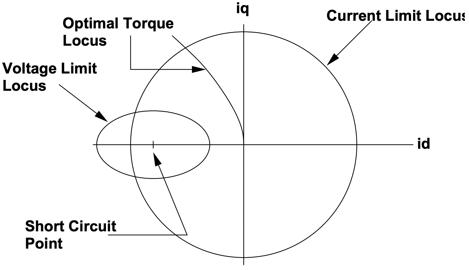Figure 7: Limits to Operation

buried magnets, \(\ L_{d}<L_{q}\), so the optimal operation of the machine will be with negative \(\ I_{d}\). We will show how to determine this optimum operation anon, but it will in general follow a curve in the \(\ I_{d}\), \(\ I_{q}\) plane as shown.

Finally, an ellipse describes the voltage limit. To start, consider what would happen if the terminals of the machine were to be short-circuited so that \(\ V=0\). If the machine is operating at sufficiently high speed so that armature resistance is negligible, armature current would be simply:

\(\ \begin{array}{l}
I_{d}=-\frac{\lambda_{f}}{L_{d}} \\
I_{q}=0
\end{array}\)

Now, loci of constant flux turn out to be ellipses around this point on the plane. Since terminal flux is proportional to voltage and inversely proportional to frequency, if the machine is operating with a given terminal voltage, the ability of that voltage to command current in the \(\ I_{d}\), \(\ I_{q}\) plane is an ellipse whose size “shrinks” as speed increases.

To simplify the mathematics involved in this estimation, we normalize reactances, fluxes, currents and torques. First, let us define the base flux to be simply \(\ \lambda_{b}=\lambda_{f}\) and the base current \(\ I_{b}\) to be the armature capability. Then we define two per-unit reactances:

\[\ x_{d}=\frac{L_{d} I_{b}}{\lambda_{b}}\label{20} \]

\[\ x_{q}=\frac{L_{q} I_{b}}{\lambda_{b}}\label{21} \]

Next, define the base torque to be:

\(\ T_{b}=p \frac{q}{2} \lambda_{b} I_{b}\)

and then, given per-unit currents \(\ i_{d}\) and \(\ i_{q}\), the per-unit torque is simply:

\[\ t_{e}=\left(1-\left(x_{q}-x_{d}\right) i_{d}\right) i_{q}\label{22} \]

It is fairly straightforward (but a bit tedious) to show that the locus of current-optimal operation (that is, the largest torque for a given current magnitude or the smallest current magnitude for a given torque) is along the curve:

\[\ i_{d}=-\sqrt{\frac{i_{a}^{2}}{2}+2\left(\frac{1}{4\left(x_{q}-x_{d}\right)}\right)^{2}-\frac{1}{2\left(x_{q}-x_{d}\right)} \sqrt{\left(\frac{1}{4\left(x_{q}-x_{d}\right)}\right)^{2}+\frac{i_{a}^{2}}{2}}}\label{23} \]

\[\ i_{q}=-\sqrt{\frac{i_{a}^{2}}{2}-2\left(\frac{1}{4\left(x_{q}-x_{d}\right)}\right)^{2}+\frac{1}{2\left(x_{q}-x_{d}\right)} \sqrt{\left(\frac{1}{4\left(x_{q}-x_{d}\right)}\right)^{2}+\frac{i_{a}^{2}}{2}}}\label{24} \]

The “rating point” will be the point along this curve when \(\ i_{a}=1\), or where this curve crosses the armature capability circle in the \(\ i_d\), \(\ i_q\) plane. It should be noted that this set of expressions only works for salient machines. For non-salient machines, of course, torque-optimal current is on the q-axis. In general, for machines with saliency, the “per-unit” torque will not be unity at the rating, so that the rated, or “Base Speed” torque is not the “Base” torque, but:

\[\ T_{r}=T_{b} \times t_{e}\label{25} \]

where \(\ t_{e}\) is calculated at the rating point (that is, \(\ i_{a}=1\) and \(\ i_{d}\) and \(\ i_{q}\) as per (23) and (24)).

For sufficiently low speeds, the power electronic drive can command the optimal current to produce torque up to rated. However, for speeds higher than the “Base Speed”, this is no longer true. Define a per-unit terminal flux:

\(\ \psi=\frac{V}{\omega \lambda_{b}}\)

Operation at a given flux magnitude implies:

\(\ \psi^{2}=\left(1+x_{d} i_{d}\right)^{2}+\left(x_{q} i_{q}\right)^{2}\)

which is an ellipse in the \(\ i_{d}\), \(\ i_{q}\) plane. The Base Speed is that speed at which this ellipse crosses the point where the optimal current curve crosses the armature capability. Operation at the highest attainable torque (for a given speed) generally implies d-axis currents that are higher than those on the optimal current locus. What is happening here is the (negative) d-axis current serves to reduce effective machine flux and hence voltage which is limiting q-axis current. Thus operation above the base speed is often referred to as “flux weakening”.

The strategy for picking the correct trajectory for current in the \(\ i_{d}\), \(\ i_{q}\) plane depends on the value of the per-unit reactance \(\ x_{d}\). For values of \(\ x_{d}>1\), it is possible to produce some torque at any speed. For values of \(\ x_{d}<1\), there is a speed for which no point in the armature current capability is within the voltage limiting ellipse, so that useful torque has gone to zero. Generally, the maximum torque operating point is the intersection of the armature current limit and the voltage limiting ellipse:

\[\ i_{d}=\frac{x_{d}}{x_{q}^{2}-x_{d}^{2}}-\sqrt{\left(\frac{x_{d}}{x_{q}^{2}-x_{d}^{2}}\right)^{2}+\frac{x_{q}^{2}-\psi^{2}+1}{x_{q}^{2}-x_{d}^{2}}}\label{26} \]

\[\ i_{q}=\sqrt{1-i_{d}^{2}}\label{27} \]

Table 1: Example Machine

D- Axis Inductance	2.53 mHy
Q- Axis Inductance	6.38 mHy
Internal Flux	58.1 mWb
Armature Current	30 A

Table 2: Operating Characteristics of Example Machine

Per-Unit D-Axis Current At Rating Point	\(\ i_{d}\)	-.5924
Per-Unit Q-Axis Current At Rating Point	\(\ i_{q}\)	.8056
Per-Unit D-Axis Reactance	\(\ x_{d}\)	1.306
Per-Unit Q-Axis Reactance	\(\ x_{q}\)	3.294
Rated Torque (Nm)	\(\ T_{r}\)	9.17
Terminal Voltage at Base Point (V)		97

It may be that there is no intersection between the armature capability and the voltage limiting ellipse. If this is the case and if \(\ x_{d}<1\), torque capability at the given speed is zero.

If, on the other hand, \(\ x_{d}>1\), it may be that the intersection between the voltage limiting ellipse and the armature current limit is not the maximum torque point. To find out, we calculate the maximum torque point on the voltage limiting ellipse. This is done in the usual way by differentiating torque with respect to \(\ i_{d}\) while holding the relationship between \(\ i_{d}\) and \(\ i_{q}\) to be on the ellipse. The algebra is a bit messy, and results in:

\[\ i_{d}=-\frac{3 x_{d}\left(x_{q}-x_{d}\right)-x_{d}^{2}}{4 x_{d}^{2}\left(x_{q}-x_{d}\right)}-\sqrt{\left(\frac{3 x_{d}\left(x_{q}-x_{d}\right)-x_{d}^{2}}{4 x_{d}^{2}\left(x_{q}-x_{d}\right)}\right)^{2}+\frac{\left(x_{q}-x_{d}\right)\left(\psi^{2}-1\right)+x_{d}}{2\left(x_{q}-x_{d}\right) x_{d}^{2}}}\label{28} \]

\[\ i_{q}=\frac{1}{x_{q}} \sqrt{\psi^{2}-\left(1+x_{d} i_{d}\right)^{2}}\label{29} \]

Ordinarily, it is probably easiest to compute (28) and (29) first, then test to see if the currents are outside the armature capability, and if they are, use (26) and (27).

These expressions give us the capability to estimate the torque-speed curve for a machine. As an example, the machine described by the parameters cited in Table 1 is a (nominal) 3 HP, 4-pole, 3000 RPM machine.

The rated operating point turns out to have the following attributes:

The loci of operation in the \(\ I_{d}\), \(\ I_{q}\) plane is shown in Figure 8. The armature current limit is shown only in the second and third quadrants, so shows up as a semicircle. The two ellipses correspond with the rated point (the larger ellipse) and with a speed that is three times rated (9000 RPM). The torque-optimal current locus can be seen running from the origin to the rating point, and the higher speed operating locus follows the armature current limit. Figure 9 shows the torque/speed and power/speed curves. Note that this sort of machine only approximates “constant power” operation at speeds above the “base” or rating point speed.

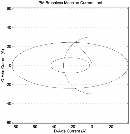Figure 8: Operating Current Loci of Example Machine

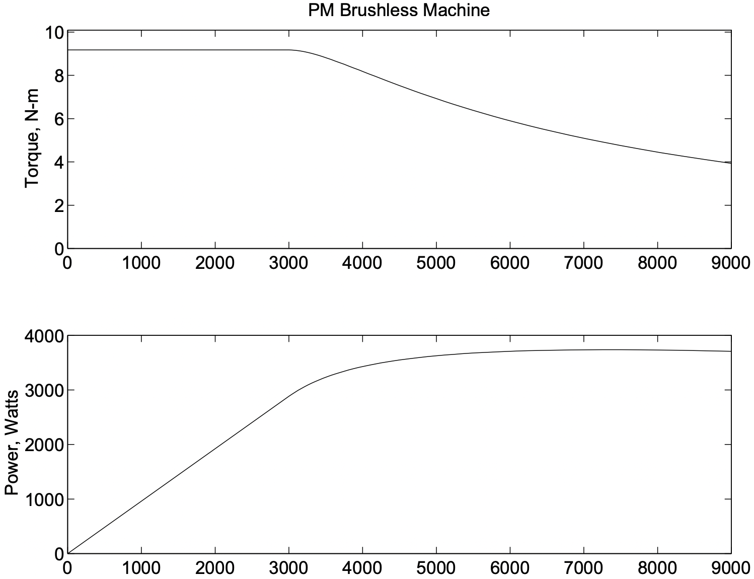Figure 9: Torque- and Power-Speed Capability