12.7: Layout

The assumed geometry is shown in Figure 11. Assumed iron (highly permeable) boundaries are at radii \(\ R_{i}\) and \(\ R_{s}\). The permanent magnets, assumed to be polarized radially and alternately (i.e. North-South ...), are located between radii \(\ R_{1}\) and \(\ R_{2}\). We assume there are \(\ p\) pole pairs (\(\ 2 p\) magnets) and that each magnet subsumes an electrical angle of \(\ \theta_{m e}\). The electrical angle is just \(\ p\) times the physical angle, so that if the magnet angle were \(\ \theta_{m e}=\pi\), the magnets would be touching.

If the magnets are arranged so that the radially polarized magnets are located around the azimuthal origin \(\ (\theta=0)\), the space fundamental of magnetization is:

\[\ \bar{M}=\bar{i}_{r} M_{0} \cos p \theta\tag{41} \]

where the fundamental magnitude is:

\[\ M_{0}=\frac{4}{\pi} \sin \frac{\theta_{m e}}{2} \frac{B_{\mathrm{rem}}}{\mu_{0}}\tag{42} \]

and \(\ B_{\text {rem }}\) is the remanent magnetization of the permanent magnet.

Since there is no current anywhere in this problem, it is convenient to treat magnetic field as the gradient of a scalar potential:

\[\ \bar{H}=-\nabla \psi\tag{43} \]

The divergence of this is:

\[\ \nabla^{2} \psi=-\nabla \cdot \bar{H}\tag{44} \]

Since magnetic flux density is divergence-free,

\[\ \nabla \cdot \bar{B}=0\tag{45} \]

we have:

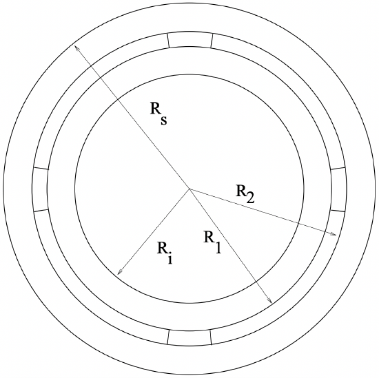Figure 11: Axial View of Magnetic Field Problem

\[\ \nabla \cdot \bar{H}=-\nabla \cdot \bar{M}\tag{46} \]

or:

\[\ \nabla^{2} \psi=\nabla \cdot \bar{M}=\frac{1}{r} M_{0} \cos p \theta\tag{47} \]

Now, if we let the magnetic scalar potential be the sum of particular and homogeneous parts:

\[\ \psi=\psi_{p}+\psi_{h}\tag{48} \]

where \(\ \nabla^{2} \psi_{h}=0\), then:

\[\ \nabla^{2} \psi_{p}=\frac{1}{r} M_{0} \cos p \theta\tag{49} \]

We can find a suitable solution to the particular part of this in the region of magnetization by trying:

\[\ \psi_{p}=C r^{\gamma} \cos p \theta\tag{50} \]

Carrying out the Laplacian on this:

\[\ \nabla^{2} \psi_{p}=C r^{\gamma-2}\left(\gamma^{2}-p^{2}\right) \cos p \theta=\frac{1}{r} M_{0} \cos p \theta\tag{51} \]

which works if \(\ \gamma=1\), in which case:

\[\ \psi_{p}=\frac{M_{0} r}{1-p^{2}} \cos p \theta\tag{52} \]

Of course this solution holds only for the region of the magnets: \(\ R_{1}<r<R_{2}\), and is zero for the regions outside of the magnets.

A suitable homogeneous solution satisfies Laplace’s equation, \(\ \nabla^{2} \psi_{h}=0\), and is in general of the form:

\[\ \psi_{h}=A r^{p} \cos p \theta+B r^{-p} \cos p \theta\tag{53} \]

Then we may write a trial total solution for the flux density as:

\[\ R_{i}<r<R_{1} \quad \psi=\left(A_{1} r^{p}+B_{1} r^{-p}\right) \cos p \theta\tag{54} \]

\[\ R_{1}<r<R_{2} \quad \psi=\left(A_{2} r^{p}+B_{2} r^{-p}+\frac{M_{0} r}{1-p^{2}}\right) \cos p \theta\tag{55} \]

\[\ R_{2}<r<R_{s} \quad \psi=\left(A_{3} r^{p}+B_{3} r^{-p}\right) \cos p \theta\tag{56} \]

The boundary conditions at the inner and outer (assumed infinitely permeable) boundaries at \(\ r=R_{i}\) and \(\ r=R_{s}\) require that the azimuthal field vanish, or \(\ \frac{\partial \psi}{\partial \theta}=0\), leading to:

\[\ B_{1}=-R_{i}^{2 p} A_{1}\tag{57} \]

\[\ B_{3}=-R_{s}^{2 p} A_{3}\tag{58} \]

At the magnet inner and outer radii, \(\ H_{\theta}\) and \(\ B_{r}\) must be continuous. These are:

\[\ H_{\theta}=-\frac{1}{r} \frac{\partial \psi}{\partial \theta}\tag{59} \]

\[\ B_{r}=\mu_{0}\left(-\frac{\partial \psi}{\partial r}+M_{r}\right)\tag{60} \]

These become, at \(\ r=R_{1}\):

\[\ -p A_{1}\left(R_{1}^{p-1}-R_{i}^{2 p} R_{1}^{-p-1}\right)=-p\left(A_{2} R_{1}^{p-1}+B_{2} R_{1}^{-p-1}\right)-p \frac{M_{0}}{1-p^{2}}\tag{61} \]

\[\ -p A_{1}\left(R_{1}^{p-1}+R_{i}^{2 p} R_{1}^{-p-1}\right)=-p\left(A_{2} R_{1}^{p-1}-B_{2} R_{1}^{-p-1}\right)-\frac{M_{0}}{1-p^{2}}+M_{0}\tag{62} \]

and at \(\ r=R_{2}\):

\[\ -p A_{3}\left(R_{2}^{p-1}-R_{s}^{2 p} R_{2}^{-p-1}\right)=-p\left(A_{2} R_{2}^{p-1}+B_{2} R_{2}^{-p-1}\right)-p \frac{M_{0}}{1-p^{2}}\tag{63} \]

\[\ -p A_{3}\left(R_{2}^{p-1}+R_{s}^{2 p} R_{2}^{-p-1}\right)=-p\left(A_{2} R_{2}^{p-1}-B_{2} R_{2}^{-p-1}\right)-\frac{M_{0}}{1-p^{2}}+M_{0}\tag{64} \]

Some small-time manipulation of these yields:

\[\ A_{1}\left(R_{1}^{p}-R_{i}^{2 p} R_{1}^{-p}\right)=A_{2} R_{1}^{p}+B_{2} R_{1}^{-p}+R_{1} \frac{M_{0}}{1-p^{2}}\tag{65} \]

\[\ A_{1}\left(R_{1}^{p}+R_{i}^{2 p} R_{1}^{-p}\right)=A_{2} R_{1}^{p}-B_{2} R_{1}^{-p}+p R_{1} \frac{M_{0}}{1-p^{2}}\tag{66} \]

\[\ A_{3}\left(R_{2}^{p}-R_{s}^{2 p} R_{2}^{-p}\right)=A_{2} R_{2}^{p}+B_{2} R_{2}^{-p}+R_{2} \frac{M_{0}}{1-p^{2}}\tag{67} \]

\[\ A_{3}\left(R_{2}^{p}+R_{s}^{2 p} R_{2}^{-p}\right)=A_{2} R_{2}^{p}-B_{2} R_{2}^{-p}+p R_{2} \frac{M_{0}}{1-p^{2}}\tag{68} \]

Taking sums and differences of the first and second and then third and fourth of these we obtain:

\[\ 2 A_{1} R_{1}^{p}=2 A_{2} R_{1}^{p}+R_{1} M_{0} \frac{1+p}{1-p^{2}}\tag{69} \]

\[\ 2 A_{1} R_{i}^{2 p} R_{1}^{-p}=-2 B_{2} R_{1}^{-p}+R_{1} M_{0} \frac{p-1}{1-p^{2}}\tag{70} \]

\[\ 2 A_{3} R_{2}^{p}=2 A_{2} R_{2}^{p}+R_{2} M_{0} \frac{1+p}{1-p^{2}}\tag{71} \]

\[\ 2 A_{3} R_{s}^{2 p} R_{2}^{-p}=-2 B_{2} R_{2}^{-p}+R_{2} M_{0} \frac{p-1}{1-p^{2}}\tag{72} \]

and then multiplying through by appropriate factors (R2 p and R1 p and then taking sums and differences of these,

\[\ \left(A_{1}-A_{3}\right) R_{1}^{p} R_{2}^{p}=\left(R_{1} R_{2}^{p}-R_{2} R_{1}^{p}\right) \frac{M_{0}}{2} \frac{p+1}{1-p^{2}}\tag{73} \]

\[\ \left(A_{1} R_{i}^{2 p}-A_{3} R_{s}^{2 p}\right) R_{1}^{-p} R_{2}^{-p}=\left(R_{1} R_{2}^{-p}-R_{2} R_{1}^{-p}\right) \frac{M_{0}}{2} \frac{p-1}{1-p^{2}}\tag{74} \]

Dividing through by the appropriate groups:

\[\ A_{1}-A_{3}=\frac{R_{1} R_{2}^{p}-R_{2} R_{1}^{p}}{R_{1}^{p} R_{2}^{p}} \frac{M_{0}}{2} \frac{1+p}{1-p^{2}}\tag{75} \]

\[\ A_{1} R_{i}^{2 p}-A_{3} R_{s}^{2 p}=\frac{R_{1} R_{2}^{-p}-R_{2} R_{1}^{-p}}{R_{1}^{-p} R_{2}^{-p}} \frac{M_{0}}{2} \frac{p-1}{1-p^{2}}\tag{76} \]

and then, by multiplying the top equation by \(\ R_{s}^{2 p}\) and subtracting:

\[\ A_{1}\left(R_{s}^{2 p}-R_{i}^{2 p}\right)=\left(\frac{R_{1} R_{2}^{p}-R_{2} R_{1}^{p}}{R_{1}^{p} R_{2}^{p}} \frac{M_{0}}{2} \frac{1+p}{1-p^{2}}\right) R_{s}^{2 p}-\frac{R_{1} R_{2}^{-p}-R_{2} R_{1}^{-p}}{R_{1}^{-p} R_{2}^{-p}} \frac{M_{0}}{2} \frac{p-1}{1-p^{2}}\tag{77} \]

This is readily solved for the field coefficients \(\ A_{1}\) and \(\ A_{3}\):

\[\ A_{1}=-\frac{M_{0}}{2\left(R_{s}^{2 p}-R_{i}^{2 p}\right)}\left(\frac{p+1}{p^{2}-1}\left(R_{1}^{1-p}-R_{2}^{1-p}\right) R_{s}^{2 p}+\frac{p-1}{p^{2}-1}\left(R_{2}^{1+p}-R_{1}^{1+p}\right)\right)\tag{78} \]

\[\ A_{3}=-\frac{M_{0}}{2\left(R_{s}^{2 p}-R_{i}^{2 p}\right)}\left(\frac{1}{1-p}\left(R_{1}^{1-p}-R_{2}^{1-p}\right) R_{i}^{2 p}-\frac{1}{1+p}\left(R_{2}^{1+p}-R_{1}^{1+p}\right)\right)\tag{79} \]

Now, noting that the scalar potential is, in region 1 (radii less than the magnet),

\(\ \psi=A_{1}\left(r^{p}-R_{i}^{2 p} r^{-p}\right) \cos p \theta \quad r<R_{1}\)

\(\ \psi=A_{3}\left(r^{p}-R_{s}^{2 p} r^{-p}\right) \cos p \theta \quad r>R_{2}\)

and noting that \(\ p(p+1) /\left(p^{2}-1\right)=p /(p-1)\) and \(\ p(p-1) /\left(p^{2}-1\right)=p /(p+1)\), magnetic field is

\(\ 80\begin{aligned}
& r<R_{1} \\
H_{r}=& \frac{M_{0}}{2\left(R_{s}^{2 p}-R_{i}^{2 p}\right)}\left(\frac{p}{p-1}\left(R_{1}^{1-p}-R_{2}^{1-p}\right) R_{s}^{2 p}+\frac{p}{p+1}\left(R_{2}^{1+p}-R_{1}^{1+p}\right)\right)\left(r^{p-1}+R_{i}^{2 p} r^{-p-1}\right) \cos p \theta \\
& r>R_{2}
\end{aligned}\)

\[\ \begin{aligned}
& r<R_{1} \\
H_{r}=& \frac{M_{0}}{2\left(R_{s}^{2 p}-R_{i}^{2 p}\right)}\left(\frac{p}{p-1}\left(R_{1}^{1-p}-R_{2}^{1-p}\right) R_{s}^{2 p}+\frac{p}{p+1}\left(R_{2}^{1+p}-R_{1}^{1+p}\right)\right)\left(r^{p-1}+R_{i}^{2 p} r^{-p-1}\right) \cos p \theta \\
& r>R_{2}
\end{aligned}\tag{80} \]

\[\ H_{r}=\frac{M_{0}}{2\left(R_{s}^{2 p}-R_{i}^{2 p}\right)}\left(\frac{p}{p-1}\left(R_{1}^{1-p}-R_{2}^{1-p}\right) R_{i}^{2 p}+\frac{p}{p+1}\left(R_{2}^{1+p}-R_{1}^{1+p}\right)\right)\left(r^{p-1}+R_{s}^{2 p} r^{-p-1}\right) \cos p \theta\tag{81} \]

The case of \(\ p=1\) appears to be a bit troublesome here, but is easily handled by noting that:

\(\ \lim _{p \rightarrow 1} \frac{p}{p-1}\left(R_{1}^{1-p}-R_{2}^{1-p}\right)=\log \frac{R_{2}}{R_{1}}\)

Now: there are a number of special cases to consider.

For the iron-free case, \(\ R_{i} \rightarrow 0\) and \(\ R_{2} \rightarrow \infty\), this becomes, simply, for \(\ r<R_{1}\)

\[\ H_{r}=\frac{M_{0}}{2} \frac{p}{p-1}\left(R_{1}^{1-p}-R_{2}^{1-p}\right) r^{p-1} \cos p \theta\tag{82} \]

Note that for the case of \(\ p=1\), the limit of this is

\(\ H_{r}=\frac{M_{0}}{2} \log \frac{R_{2}}{R_{1}} \cos \theta\)

and for \(\ r>R_{2}\):

\(\ H_{r}=\frac{M_{0}}{2} \frac{p}{p+1}\left(R_{2}^{p+1}-R_{1}^{p+1}\right) r^{-(p+1)} \cos p \theta\)

For the case of a machine with iron boundaries and windings in slots, we are interested in the fields at the boundaries. In such a case, usually, either \(\ R_{i}=R_{1}\) or \(\ R_{s}=R_{2}\). The fields are:

at the outer boundary: \(\ r=R_{s}\):

\(\ H_{r}=M_{0} \frac{R_{s}^{p-1}}{R_{s}^{2 p}-R_{i}^{2 p}}\left(\frac{p}{p+1}\left(R_{2}^{p+1}-R_{1}^{p+1}\right)+\frac{p}{p-1} R_{i}^{2 p}\left(R_{1}^{1-p}-R_{2}^{1-p}\right)\right) \cos p \theta\)

or at the inner boundary: \(\ r=R_{i}\):

\(\ H_{r}=M_{0} \frac{R_{i}^{p-1}}{R_{s}^{2 p}-R_{i}^{2 p}}\left(\frac{p}{p+1}\left(R_{2}^{p+1}-R_{1}^{p+1}\right)+\frac{p}{p-1} R_{s}^{2 p}\left(R_{1}^{1-p}-R_{2}^{1-p}\right)\right) \cos p \theta\)