

1.2: Pulse Characteristics
- Page ID
- 44639

\( \newcommand{\vecs}[1]{\overset { \scriptstyle \rightharpoonup} {\mathbf{#1}} } \)
\( \newcommand{\vecd}[1]{\overset{-\!-\!\rightharpoonup}{\vphantom{a}\smash {#1}}} \)
\( \newcommand{\dsum}{\displaystyle\sum\limits} \)
\( \newcommand{\dint}{\displaystyle\int\limits} \)
\( \newcommand{\dlim}{\displaystyle\lim\limits} \)
\( \newcommand{\id}{\mathrm{id}}\) \( \newcommand{\Span}{\mathrm{span}}\)
( \newcommand{\kernel}{\mathrm{null}\,}\) \( \newcommand{\range}{\mathrm{range}\,}\)
\( \newcommand{\RealPart}{\mathrm{Re}}\) \( \newcommand{\ImaginaryPart}{\mathrm{Im}}\)
\( \newcommand{\Argument}{\mathrm{Arg}}\) \( \newcommand{\norm}[1]{\| #1 \|}\)
\( \newcommand{\inner}[2]{\langle #1, #2 \rangle}\)
\( \newcommand{\Span}{\mathrm{span}}\)
\( \newcommand{\id}{\mathrm{id}}\)
\( \newcommand{\Span}{\mathrm{span}}\)
\( \newcommand{\kernel}{\mathrm{null}\,}\)
\( \newcommand{\range}{\mathrm{range}\,}\)
\( \newcommand{\RealPart}{\mathrm{Re}}\)
\( \newcommand{\ImaginaryPart}{\mathrm{Im}}\)
\( \newcommand{\Argument}{\mathrm{Arg}}\)
\( \newcommand{\norm}[1]{\| #1 \|}\)
\( \newcommand{\inner}[2]{\langle #1, #2 \rangle}\)
\( \newcommand{\Span}{\mathrm{span}}\) \( \newcommand{\AA}{\unicode[.8,0]{x212B}}\)
\( \newcommand{\vectorA}[1]{\vec{#1}} % arrow\)
\( \newcommand{\vectorAt}[1]{\vec{\text{#1}}} % arrow\)
\( \newcommand{\vectorB}[1]{\overset { \scriptstyle \rightharpoonup} {\mathbf{#1}} } \)
\( \newcommand{\vectorC}[1]{\textbf{#1}} \)
\( \newcommand{\vectorD}[1]{\overrightarrow{#1}} \)
\( \newcommand{\vectorDt}[1]{\overrightarrow{\text{#1}}} \)
\( \newcommand{\vectE}[1]{\overset{-\!-\!\rightharpoonup}{\vphantom{a}\smash{\mathbf {#1}}}} \)
\( \newcommand{\vecs}[1]{\overset { \scriptstyle \rightharpoonup} {\mathbf{#1}} } \)
\(\newcommand{\longvect}{\overrightarrow}\)
\( \newcommand{\vecd}[1]{\overset{-\!-\!\rightharpoonup}{\vphantom{a}\smash {#1}}} \)
\(\newcommand{\ket}[1]{\left| #1 \right>}\)
\(\newcommand{\bra}[1]{\left< #1 \right|}\)
\(\newcommand{\braket}[2]{\left< #1 \vphantom{#2} \right| \left. #2 \vphantom{#1} \right>}\)
\(\newcommand{\braopket}[3]{\left< #1 \vphantom{#2}\vphantom{#3} \right| #2 \vphantom{#1}\vphantom{#3} \left| #3 \vphantom{#1}\vphantom{#2} \right>}\)
\(\newcommand{\qmvec}[1]{\mathbf{\vec{#1}}}\)
\(\newcommand{\op}[1]{\hat{\mathbf{#1}}}\)
\(\newcommand{\expect}[1]{\langle #1 \rangle}\)
\(\newcommand{\dfn}[1]{\emph{\textbf{#1}}}\)
Most often, there is not an isolated pulse, but rather a pulse train.
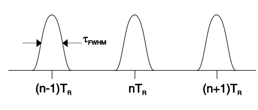
\(T_R\): pulse repetition time
\(W\) : pulse energy
\(P_{ave} = W/T_R\): average power
\(\tau{\text{FWHM}}\) is the Full Width at Half Maximum of the intensity envelope of the pulse in the time domain.
The peak power is given by
\[P_p = \dfrac{W}{\tau{\text{FWHM}}} = P_{ave} \dfrac{T_R}{\tau{\text{FWHM}}} \nonumber \]
and the peak electric field is given by
\[E_p = \sqrt{2 Z_{F_0} \dfrac{P_p}{A_{\text{eff}}} \nonumber \]
\(A_{\text{eff}}\) is the beam cross-section and \(Z_{F_0} = 377 \Omega\) is the free space impedance.
Time scales:
\[\begin{array} {lcl} {\text{1 ns}} & \sim & {30\text{ cm (high-speed electronics, GHz}} \\ {\text{1 ps}} & \sim & {300\ \mu\text{m}} \\ {\text{1 fs}} & \sim & {\text{300 nm}} \\ {1 \text{ as} = 10^{-18} s} & \sim & {\text{0.3 nm = 3} \mathring{A} \text{ (typ-lattice constant in metal)}} \end{array} \nonumber \]
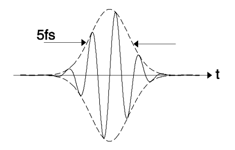
The shortest pulses generated to date are about 4 - 5 fs at 800 nm \((\lambda/c = 2.7\) fs), less than two optical cycles and 250 as at 25 nm. For few-cycle pulses, the electric field becomes important, not only the intensity!
average power:
\[\begin{array} {cl} {P_{ave} \sim} & {\text{1W, up to 100 W in progress.}} \\ {\ } & {\text{kW possible, not yet pulsed}} \end{array} \nonumber \]
repetition rates:
\[T_R^{-1} = f_R = \text{m Hz - 100 GHz}\nonumber \]
pulse energy:
\[W = 1pJ - 1kJ\nonumber \]
pulse width:
\[\tau_{\text{FWHM}} = \begin{array} {ll} {\text{5 fs - 50 ps,}} & {\text{modelocked}} \\ {\text{30 ps - 100 ns,}} & {\text{Q - switched}} \end{array}\nonumber \]
peak power:
\[P_p = \dfrac{\text{1 kJ}}{\text{1 ps}} \sim \text{1 PW},\nonumber \]
obtained with Nd:glass (LLNL - USA, [1][2][3]).
For a typical lab pulse, the peak power is
\[P_p = \dfrac{\text{10 nJ}}{\text{10 fs}} \sim \text{1 MW}\nonumber \]
peak field of typical lab pulse:
\[E_p = \sqrt{2 \times 377 \times \dfrac{10^6 \times 10^{12}}{\pi \times (1.5)^2}} \dfrac{\text{V}}{\text{m}} \approx 10^{10} \dfrac{\text{V}}{\text{m}} = \dfrac{10\text{V}}{\text{nm}}\nonumber \]