1.3: Basic Fourier Analysis
- Page ID
- 25162
\( \newcommand{\vecs}[1]{\overset { \scriptstyle \rightharpoonup} {\mathbf{#1}} } \)
\( \newcommand{\vecd}[1]{\overset{-\!-\!\rightharpoonup}{\vphantom{a}\smash {#1}}} \)
\( \newcommand{\id}{\mathrm{id}}\) \( \newcommand{\Span}{\mathrm{span}}\)
( \newcommand{\kernel}{\mathrm{null}\,}\) \( \newcommand{\range}{\mathrm{range}\,}\)
\( \newcommand{\RealPart}{\mathrm{Re}}\) \( \newcommand{\ImaginaryPart}{\mathrm{Im}}\)
\( \newcommand{\Argument}{\mathrm{Arg}}\) \( \newcommand{\norm}[1]{\| #1 \|}\)
\( \newcommand{\inner}[2]{\langle #1, #2 \rangle}\)
\( \newcommand{\Span}{\mathrm{span}}\)
\( \newcommand{\id}{\mathrm{id}}\)
\( \newcommand{\Span}{\mathrm{span}}\)
\( \newcommand{\kernel}{\mathrm{null}\,}\)
\( \newcommand{\range}{\mathrm{range}\,}\)
\( \newcommand{\RealPart}{\mathrm{Re}}\)
\( \newcommand{\ImaginaryPart}{\mathrm{Im}}\)
\( \newcommand{\Argument}{\mathrm{Arg}}\)
\( \newcommand{\norm}[1]{\| #1 \|}\)
\( \newcommand{\inner}[2]{\langle #1, #2 \rangle}\)
\( \newcommand{\Span}{\mathrm{span}}\) \( \newcommand{\AA}{\unicode[.8,0]{x212B}}\)
\( \newcommand{\vectorA}[1]{\vec{#1}} % arrow\)
\( \newcommand{\vectorAt}[1]{\vec{\text{#1}}} % arrow\)
\( \newcommand{\vectorB}[1]{\overset { \scriptstyle \rightharpoonup} {\mathbf{#1}} } \)
\( \newcommand{\vectorC}[1]{\textbf{#1}} \)
\( \newcommand{\vectorD}[1]{\overrightarrow{#1}} \)
\( \newcommand{\vectorDt}[1]{\overrightarrow{\text{#1}}} \)
\( \newcommand{\vectE}[1]{\overset{-\!-\!\rightharpoonup}{\vphantom{a}\smash{\mathbf {#1}}}} \)
\( \newcommand{\vecs}[1]{\overset { \scriptstyle \rightharpoonup} {\mathbf{#1}} } \)
\( \newcommand{\vecd}[1]{\overset{-\!-\!\rightharpoonup}{\vphantom{a}\smash {#1}}} \)
\(\newcommand{\avec}{\mathbf a}\) \(\newcommand{\bvec}{\mathbf b}\) \(\newcommand{\cvec}{\mathbf c}\) \(\newcommand{\dvec}{\mathbf d}\) \(\newcommand{\dtil}{\widetilde{\mathbf d}}\) \(\newcommand{\evec}{\mathbf e}\) \(\newcommand{\fvec}{\mathbf f}\) \(\newcommand{\nvec}{\mathbf n}\) \(\newcommand{\pvec}{\mathbf p}\) \(\newcommand{\qvec}{\mathbf q}\) \(\newcommand{\svec}{\mathbf s}\) \(\newcommand{\tvec}{\mathbf t}\) \(\newcommand{\uvec}{\mathbf u}\) \(\newcommand{\vvec}{\mathbf v}\) \(\newcommand{\wvec}{\mathbf w}\) \(\newcommand{\xvec}{\mathbf x}\) \(\newcommand{\yvec}{\mathbf y}\) \(\newcommand{\zvec}{\mathbf z}\) \(\newcommand{\rvec}{\mathbf r}\) \(\newcommand{\mvec}{\mathbf m}\) \(\newcommand{\zerovec}{\mathbf 0}\) \(\newcommand{\onevec}{\mathbf 1}\) \(\newcommand{\real}{\mathbb R}\) \(\newcommand{\twovec}[2]{\left[\begin{array}{r}#1 \\ #2 \end{array}\right]}\) \(\newcommand{\ctwovec}[2]{\left[\begin{array}{c}#1 \\ #2 \end{array}\right]}\) \(\newcommand{\threevec}[3]{\left[\begin{array}{r}#1 \\ #2 \\ #3 \end{array}\right]}\) \(\newcommand{\cthreevec}[3]{\left[\begin{array}{c}#1 \\ #2 \\ #3 \end{array}\right]}\) \(\newcommand{\fourvec}[4]{\left[\begin{array}{r}#1 \\ #2 \\ #3 \\ #4 \end{array}\right]}\) \(\newcommand{\cfourvec}[4]{\left[\begin{array}{c}#1 \\ #2 \\ #3 \\ #4 \end{array}\right]}\) \(\newcommand{\fivevec}[5]{\left[\begin{array}{r}#1 \\ #2 \\ #3 \\ #4 \\ #5 \\ \end{array}\right]}\) \(\newcommand{\cfivevec}[5]{\left[\begin{array}{c}#1 \\ #2 \\ #3 \\ #4 \\ #5 \\ \end{array}\right]}\) \(\newcommand{\mattwo}[4]{\left[\begin{array}{rr}#1 \amp #2 \\ #3 \amp #4 \\ \end{array}\right]}\) \(\newcommand{\laspan}[1]{\text{Span}\{#1\}}\) \(\newcommand{\bcal}{\cal B}\) \(\newcommand{\ccal}{\cal C}\) \(\newcommand{\scal}{\cal S}\) \(\newcommand{\wcal}{\cal W}\) \(\newcommand{\ecal}{\cal E}\) \(\newcommand{\coords}[2]{\left\{#1\right\}_{#2}}\) \(\newcommand{\gray}[1]{\color{gray}{#1}}\) \(\newcommand{\lgray}[1]{\color{lightgray}{#1}}\) \(\newcommand{\rank}{\operatorname{rank}}\) \(\newcommand{\row}{\text{Row}}\) \(\newcommand{\col}{\text{Col}}\) \(\renewcommand{\row}{\text{Row}}\) \(\newcommand{\nul}{\text{Nul}}\) \(\newcommand{\var}{\text{Var}}\) \(\newcommand{\corr}{\text{corr}}\) \(\newcommand{\len}[1]{\left|#1\right|}\) \(\newcommand{\bbar}{\overline{\bvec}}\) \(\newcommand{\bhat}{\widehat{\bvec}}\) \(\newcommand{\bperp}{\bvec^\perp}\) \(\newcommand{\xhat}{\widehat{\xvec}}\) \(\newcommand{\vhat}{\widehat{\vvec}}\) \(\newcommand{\uhat}{\widehat{\uvec}}\) \(\newcommand{\what}{\widehat{\wvec}}\) \(\newcommand{\Sighat}{\widehat{\Sigma}}\) \(\newcommand{\lt}{<}\) \(\newcommand{\gt}{>}\) \(\newcommand{\amp}{&}\) \(\definecolor{fillinmathshade}{gray}{0.9}\)The Fourier theorem, named after the French mathematician Jean-Baptiste Joseph Fourier, states that any repetitive waveform can be represented as a collection of sine and cosine waves of the proper amplitude and frequency. Alternately, it may be represented as a series of sine waves each with the proper amplitude, frequency and phase. This includes complex signals such as the human voice and musical instruments. Consequently, if a system is linear, the response of a system to a complex wave may be understood in terms of its response to individual sine waves, via superposition.
In this collection of waves, each component is known as a partial with the lowest frequency component known as the fundamental. All other partials are grouped together and referred to as overtones. “Regular” waveforms such as square waves and triangle waves feature a harmonic overtone sequence meaning that these overtones are integer multiples of the fundamental. As a shortcut, they are often referred to as just harmonics.
It might be hard to visualize initially, but like all waves, waves in the shape of a square or triangle are made up of a series of sines. The equation for a square wave is:
\[v(t) = \sum_{n=1}^{\infty} \frac{1}{2n-1} \sin ((2n-1)2 \pi ft) \label{1.4} \]
This says that a square wave of frequency \(f\) is made up of an infinite series of sines at odd integer multiples of \(f\), with an inverse amplitude characteristic. For example, a 100 Hz square consists of a 100 Hz sine, plus a 300 Hz sine at 1/3 amplitude, plus a 500 Hz sine at 1/5 amplitude, plus a 700 Hz sine at 1/7 amplitude, and so on.
A triangle wave is similar:
\[v(t) = \sum_{n=1}^{\infty} \frac{1}{(2n-1)^2} \cos ((2n-1)2 \pi ft) \label{1.5} \]
Thus a triangle wave of frequency \(f\) is made up of an infinite series of cosines (sines with a 90 degree or one quarter cycle phase shift) at odd integer multiples of \(f\), with an inverse square amplitude characteristic. For example, a 100 Hz triangle consists of a 100 Hz cosine, plus a 300 Hz cosine at 1/9 amplitude, plus a 500 Hz cosine at 1/25 amplitude, plus a 700 Hz cosine at 1/49 amplitude, and so on.
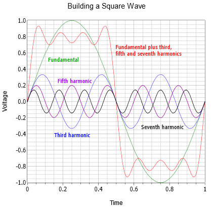
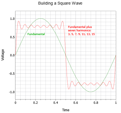
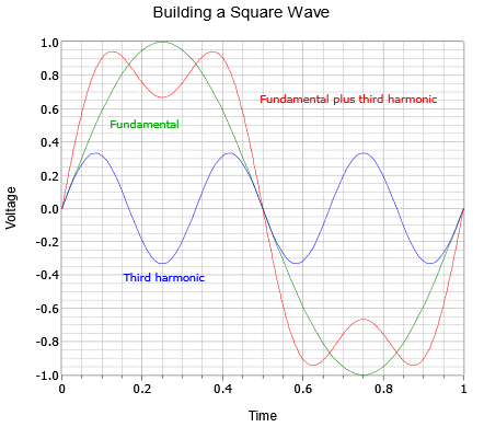
A series of graphs showing the construction of a square wave and a triangle wave follow. The square wave sequence begins with the fundamental and the first harmonic in Figure \(\PageIndex{1}\). The result is an oddly bumpy wave. The second graph of Figure \(\PageIndex{2}\) adds the next two harmonics. As more harmonics are added, the sides get steeper and the top/bottom start to flatten. They flatten because each additional harmonic partially cancels some of the peaks and valleys from the previous summation. This gives rise to a greater number of undulations with each undulation being smaller in amplitude. The sequence finishes with Figure \(\PageIndex{3}\) showing seven harmonics being added with the result approaching a reasonable square wave. As ever more harmonics are added, the wave would approach a flat top and bottom with vertical sides, the idealized square wave.
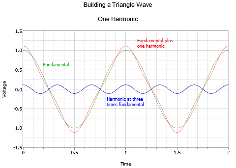
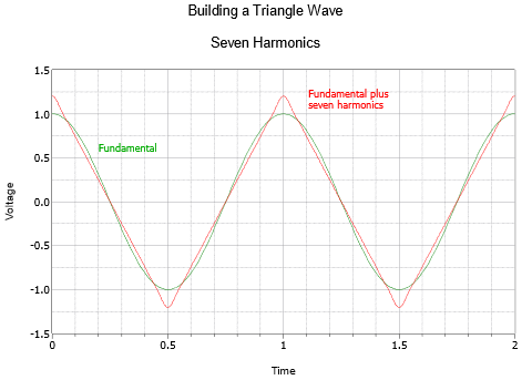
The triangle sequence begins with a fundamental and the first harmonic as shown in Figure \(\PageIndex{4}\). The resulting combination is already trending away from a simple sine shape. The second and final graph, Figure \(\PageIndex{5}\), shows a total of seven harmonics. The result is very close to a triangle, the only obvious deviation is the slight rounding at the very peaks. The addition of more harmonics would cause these to sharpen further.