10.4: Combining the Elements - Multi-Stage Effects
- Page ID
- 25170
\( \newcommand{\vecs}[1]{\overset { \scriptstyle \rightharpoonup} {\mathbf{#1}} } \)
\( \newcommand{\vecd}[1]{\overset{-\!-\!\rightharpoonup}{\vphantom{a}\smash {#1}}} \)
\( \newcommand{\id}{\mathrm{id}}\) \( \newcommand{\Span}{\mathrm{span}}\)
( \newcommand{\kernel}{\mathrm{null}\,}\) \( \newcommand{\range}{\mathrm{range}\,}\)
\( \newcommand{\RealPart}{\mathrm{Re}}\) \( \newcommand{\ImaginaryPart}{\mathrm{Im}}\)
\( \newcommand{\Argument}{\mathrm{Arg}}\) \( \newcommand{\norm}[1]{\| #1 \|}\)
\( \newcommand{\inner}[2]{\langle #1, #2 \rangle}\)
\( \newcommand{\Span}{\mathrm{span}}\)
\( \newcommand{\id}{\mathrm{id}}\)
\( \newcommand{\Span}{\mathrm{span}}\)
\( \newcommand{\kernel}{\mathrm{null}\,}\)
\( \newcommand{\range}{\mathrm{range}\,}\)
\( \newcommand{\RealPart}{\mathrm{Re}}\)
\( \newcommand{\ImaginaryPart}{\mathrm{Im}}\)
\( \newcommand{\Argument}{\mathrm{Arg}}\)
\( \newcommand{\norm}[1]{\| #1 \|}\)
\( \newcommand{\inner}[2]{\langle #1, #2 \rangle}\)
\( \newcommand{\Span}{\mathrm{span}}\) \( \newcommand{\AA}{\unicode[.8,0]{x212B}}\)
\( \newcommand{\vectorA}[1]{\vec{#1}} % arrow\)
\( \newcommand{\vectorAt}[1]{\vec{\text{#1}}} % arrow\)
\( \newcommand{\vectorB}[1]{\overset { \scriptstyle \rightharpoonup} {\mathbf{#1}} } \)
\( \newcommand{\vectorC}[1]{\textbf{#1}} \)
\( \newcommand{\vectorD}[1]{\overrightarrow{#1}} \)
\( \newcommand{\vectorDt}[1]{\overrightarrow{\text{#1}}} \)
\( \newcommand{\vectE}[1]{\overset{-\!-\!\rightharpoonup}{\vphantom{a}\smash{\mathbf {#1}}}} \)
\( \newcommand{\vecs}[1]{\overset { \scriptstyle \rightharpoonup} {\mathbf{#1}} } \)
\( \newcommand{\vecd}[1]{\overset{-\!-\!\rightharpoonup}{\vphantom{a}\smash {#1}}} \)
\(\newcommand{\avec}{\mathbf a}\) \(\newcommand{\bvec}{\mathbf b}\) \(\newcommand{\cvec}{\mathbf c}\) \(\newcommand{\dvec}{\mathbf d}\) \(\newcommand{\dtil}{\widetilde{\mathbf d}}\) \(\newcommand{\evec}{\mathbf e}\) \(\newcommand{\fvec}{\mathbf f}\) \(\newcommand{\nvec}{\mathbf n}\) \(\newcommand{\pvec}{\mathbf p}\) \(\newcommand{\qvec}{\mathbf q}\) \(\newcommand{\svec}{\mathbf s}\) \(\newcommand{\tvec}{\mathbf t}\) \(\newcommand{\uvec}{\mathbf u}\) \(\newcommand{\vvec}{\mathbf v}\) \(\newcommand{\wvec}{\mathbf w}\) \(\newcommand{\xvec}{\mathbf x}\) \(\newcommand{\yvec}{\mathbf y}\) \(\newcommand{\zvec}{\mathbf z}\) \(\newcommand{\rvec}{\mathbf r}\) \(\newcommand{\mvec}{\mathbf m}\) \(\newcommand{\zerovec}{\mathbf 0}\) \(\newcommand{\onevec}{\mathbf 1}\) \(\newcommand{\real}{\mathbb R}\) \(\newcommand{\twovec}[2]{\left[\begin{array}{r}#1 \\ #2 \end{array}\right]}\) \(\newcommand{\ctwovec}[2]{\left[\begin{array}{c}#1 \\ #2 \end{array}\right]}\) \(\newcommand{\threevec}[3]{\left[\begin{array}{r}#1 \\ #2 \\ #3 \end{array}\right]}\) \(\newcommand{\cthreevec}[3]{\left[\begin{array}{c}#1 \\ #2 \\ #3 \end{array}\right]}\) \(\newcommand{\fourvec}[4]{\left[\begin{array}{r}#1 \\ #2 \\ #3 \\ #4 \end{array}\right]}\) \(\newcommand{\cfourvec}[4]{\left[\begin{array}{c}#1 \\ #2 \\ #3 \\ #4 \end{array}\right]}\) \(\newcommand{\fivevec}[5]{\left[\begin{array}{r}#1 \\ #2 \\ #3 \\ #4 \\ #5 \\ \end{array}\right]}\) \(\newcommand{\cfivevec}[5]{\left[\begin{array}{c}#1 \\ #2 \\ #3 \\ #4 \\ #5 \\ \end{array}\right]}\) \(\newcommand{\mattwo}[4]{\left[\begin{array}{rr}#1 \amp #2 \\ #3 \amp #4 \\ \end{array}\right]}\) \(\newcommand{\laspan}[1]{\text{Span}\{#1\}}\) \(\newcommand{\bcal}{\cal B}\) \(\newcommand{\ccal}{\cal C}\) \(\newcommand{\scal}{\cal S}\) \(\newcommand{\wcal}{\cal W}\) \(\newcommand{\ecal}{\cal E}\) \(\newcommand{\coords}[2]{\left\{#1\right\}_{#2}}\) \(\newcommand{\gray}[1]{\color{gray}{#1}}\) \(\newcommand{\lgray}[1]{\color{lightgray}{#1}}\) \(\newcommand{\rank}{\operatorname{rank}}\) \(\newcommand{\row}{\text{Row}}\) \(\newcommand{\col}{\text{Col}}\) \(\renewcommand{\row}{\text{Row}}\) \(\newcommand{\nul}{\text{Nul}}\) \(\newcommand{\var}{\text{Var}}\) \(\newcommand{\corr}{\text{corr}}\) \(\newcommand{\len}[1]{\left|#1\right|}\) \(\newcommand{\bbar}{\overline{\bvec}}\) \(\newcommand{\bhat}{\widehat{\bvec}}\) \(\newcommand{\bperp}{\bvec^\perp}\) \(\newcommand{\xhat}{\widehat{\xvec}}\) \(\newcommand{\vhat}{\widehat{\vvec}}\) \(\newcommand{\uhat}{\widehat{\uvec}}\) \(\newcommand{\what}{\widehat{\wvec}}\) \(\newcommand{\Sighat}{\widehat{\Sigma}}\) \(\newcommand{\lt}{<}\) \(\newcommand{\gt}{>}\) \(\newcommand{\amp}{&}\) \(\definecolor{fillinmathshade}{gray}{0.9}\)A complete gain or phase plot combines three elements: (1) the midband response, (2) the lead response, and (3) the lag response. Normally, a particular design will contain multiple lead and lag networks. The complete response is the summation of the individual responses. For this reason, it is useful to find the dominant lead and lag networks. These are the networks that affect the midband response first. For lead networks, the dominant one will be the one with the highest \(f_c\). Conversely, the dominant lag network will be the one with the lowest \(f_c\). It is very common to approximate the complete system response by drawing straight-line segments such as those given in Figures 10.3.2 and 10.3.4. The process goes something like this:
- Locate all \(f_c\)s on the frequency axis.
- Draw a straight line between the dominant lag and lead \(f_c\)s at the midband gain. If the system does not contain any lead networks, continue the midband gain line down to DC.
- Draw a 6 dB per octave slope between the dominant lead and the next lower lead network.
- Because the effects of the networks are cumulative, draw a 12 dB per octave slope between the second lead \(f_c\) and the third \(f_c\). After the third \(f_c\), the slope should be 18 dB per octave, after the fourth, 24 dB per octave, and so on.
- Draw a −6 dB per octave slope between the dominant lag \(f_c\) and the next highest \(f_c\). Again, the effects are cumulative, so increase the slope by −6 dB at every new \(f_c\).
Example \(\PageIndex{1}\)
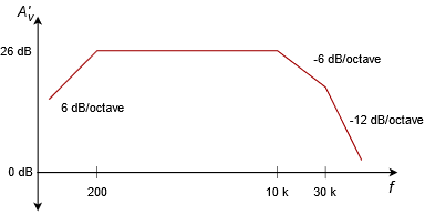
Draw the Bode gain plot for the following amplifier: \(A'_v\) midband = 26 dB, one lead network critical at 200 Hz, one lag network critical at 10 kHz, and another lag network critical at 30 kHz.
The dominant lag network is 10 kHz. There is only one lead network, so it’s dominant by default.
- Draw a straight line between 200 Hz and 10 kHz at an amplitude of 26 dB.
- Draw a 6 dB per octave slope below 200 Hz. To do this, drop down one octave (100 Hz) and subtract 6 dB from the present gain (26 dB − 6dB = 20 dB.) The line will start at the point 200 Hz/26 dB, and pass through the point 100 Hz/20 dB. Because there are no other lead networks, this line may be extended to the left edge of the graph.
- Draw a −6 dB per octave slope between 10 kHz and 30 kHz. The construction point will be 20 kHz/20 dB. Continue this line to 30 kHz. The gain at the 30 kHz intersection should be around 16 dB. The slope above this second \(f_c\) will be −12 dB per octave. Therefore, the second construction point should be at 60 kHz/4 dB (one octave above 30 kHz, and 12 dB down from the 30 kHz gain). Because this is the final lag network, this line may be extended to the right edge of the graph.
A completed graph is shown in Figure \(\PageIndex{1}\).

There is one item that should be noted before we leave this section, and that is the concept of narrowing. Narrowing occurs when two or more networks share similar critical frequencies, and one of them is a dominant network. The result is that the true −3 dB breakpoints may be altered. Here is an extreme example. Assume that a circuit has two lag networks, both critical at 1 MHz. A Bode plot would indicate that the breakpoint is 1 MHz. This is not really true. Remember, the effects of lead and lag networks are cumulative. Because each network produces a 3 dB loss at 1 MHz, the net loss at this frequency is actually 6 dB. The true −3 dB point will have been shifted. The Bode plot only gives you the approximate shape of the response.


