5.4: Microstrip Operating Frequency Limitations

The higher-order modes, i.e. other than the quasi-TEM mode, with the lowest cut-off or critical frequency, \(f_{c}\) are usually (a) the lowest-order TM mode and (b) the lowest-order transverse microstrip resonance mode.

5.4.1 Microstrip Dielectric Mode (Slab Mode)

A dielectric on a ground plane with an air region (of a wavelength or more above it) can support a TM mode, variously called a microstrip dielectric mode, substrate mode, microstrip TM mode, or slab mode. Referring to Figure 5.3.4(b), the cut-off or critical frequency, \(f_{c,\text{SLAB}}\) above which the slab mode exists is when the distance between the electric and magnetic walls \(h > \lambda /4\), where \(\lambda = \lambda_{0}/\sqrt{\varepsilon_{r}}\) is the wavelength in the dielectric, so

\[\label{eq:1} f_{c,\text{SLAB}}=\frac{c}{4h\sqrt{\varepsilon_{r}}} \]

Experience is that the the critical frequency is less than this, e.g. \(20\%\) less, which is consistent with the distance between the electric and magnetic walls being slightly larger so that the magnetic wall is slightly into the air region. The critical frequency is also affected by discontinuities. This stresses the importance of measurements of a design in development and the design engineer aware of effects such as multimoding that are not fully accounted for in modeling. No software can properly account for all effects in part because EM simulation tools rely on symmetry, smooth surface, and dielectrics and conductors with uniform properties.

Example \(\PageIndex{1}\): Dielectric Mode

The strip of a microstrip has a width of \(1\text{ mm}\) and the substrate is \(2.5\text{ mm}\) thick with a relative permittivity of \(9\). What is the lowest frequency that slab mode exists?

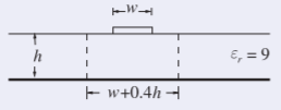
Figure \(\PageIndex{1}\)

Solution

The critical frequency comes from the thickness and permittivity of the substrate. The slab mode exists when a variation of the magnetic or electric field can be supported between the ground plane and the approximate magnetic wall at the substrate/air interface. This is when \(h =\frac{1}{4}\lambda = \lambda_{0}/(4\sqrt{9}) = 2.5\text{ mm} ⇒\lambda_{0} = 3\text{ cm}\). Thus the critical slab mode critical frequency is

\[f_{c,\text{SLAB}}=10\text{ GHz}\nonumber \]

5.4.2 Higher-Order Microstrip Mode

The next highest microstrip mode (or parallel-plate TE mode) above the quasi-TEM mode occurs when there is a half-sinusoidal variation of the electric field between the strip and the ground plane. This corresponds to Figure 5.3.4(a). However the first higher-order microstrip mode has been found be experiemntally found to exist at a lower frequency than derived using the parallel electrical wall model. This is because the microstrip fields do not follow the shortest distance between the strip and the ground plane. Thus the fields along the longer paths to the sides of the strip can vary at a lower frequency than on the direct path. With experimental support it has been established that the first higher-order microstrip mode can exist at frequencies above [2].

\[\label{eq:2} f_{\text{Higher - Microstrip}}=\frac{c}{4h\sqrt{\varepsilon_{r}-1}} \]

Example \(\PageIndex{2}\): Higher-Order Microstrip Mode

The strip of a microstrip has a width of \(1\text{ mm}\) and is fabricated on a lossless substrate that is \(2.5\text{ mm}\) thick and has a relative permittivity of \(9\). At what frequency does the first higher microstrip mode first propagate?

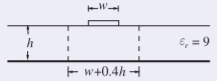
Figure \(\PageIndex{2}\)

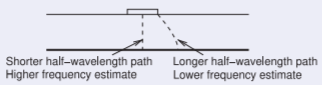
Figure \(\PageIndex{3}\)

Solution

The higher-order microstrip mode occurs when a half-wavelength variation of the electric field between the strip and the ground plane can be supported. When \(h = \lambda /2 = \lambda_{0}/(3\cdot 2) = 2.5\text{ mm}\); that is, the mode will occur when \(\lambda_{0} = 15\text{ mm}\). So

\[f_{\text{Higher - Microstrip}}=20\text{ GHz}\nonumber \]

A better estimate of the frequency where the higher-order microstrip mode becomes a problem is given by Equation \(\eqref{eq:2}\):

\[f_{\text{Higher - Microstrip}}=c/(4h\sqrt{\varepsilon_{r}-1})=10.6\text{ GHz}\nonumber \]

So two estimates have been calculated for the frequency at which the first higher-order microstrip mode can first exist. The first estimate is approximate and is based on a half-wavelength variation of the electric field confined to the direct path between the strip and the ground plane. The second estimate is more accurate as it considers that on the edge of the strip the fields follow a longer path to the ground plane. It is the half-wavelength variation on this longer path that determines if the higher-order microstrip mode will exist.

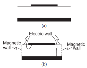
Figure \(\PageIndex{4}\): Approximation of a microstrip line as a waveguide: (a) cross section of microstrip; and (b) microstrip waveguide model having effective width \(w + 0.4h\) with magnetic and electric walls.

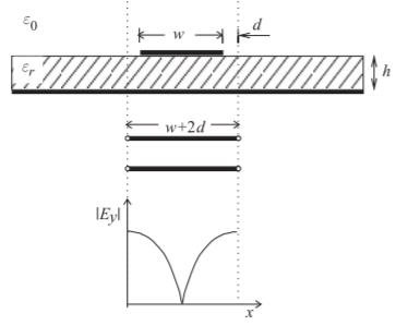
Figure \(\PageIndex{5}\): Transverse resonance: standing wave (\(|E_{y}|\)) and equivalent transmission line of length \(w + 2d\), where \(d = 0.2h\).

5.4.3 Transverse Microstrip Resonance

For a wide microstrip line, a transverse resonance mode can exist. This is the mode that occurs when EM energy bounces between the edges of the strip, see Figure \(\PageIndex{4}\). Here the microstrip is modelled by magnetic walls on the sides and an extended electrical wall on the top surface of the dielectric. The transverse resonance mode corresponds to the lowest order \(H\) field variation between the magnetic walls. The equivalent circuit for the transverse-resonant mode is a resonant transmission line of length \(w + 2d\), as shown in Figure \(\PageIndex{5}\), where \(d = 0.2h\) accounts for the microstrip side fringing. A half-wavelength must be supported by the length \(w + 2d\). Therefore the cutoff half-wavelength is

\[\label{eq:3}\frac{\lambda_{c}}{2}=w+2d=w+0.4h,\quad\text{that is,}\quad\frac{c}{2f_{c}\sqrt{\varepsilon_{r}}}=w+0.4h \]

Hence the critical frequency for transverse resonance is

\[\label{eq:4}f_{c,\text{TRAN}}=\frac{c}{\sqrt{\varepsilon_{r}}(2w+0.8h)} \]

Example \(\PageIndex{3}\): Transverse Resonance Mode

The strip of a microstrip has a width of \(1\text{ mm}\) and is fabricated on a lossless substrate that is \(2.5\text{ mm}\) thick and has a relative permittivity of \(9\).

1. At what frequency does the transverse resonance first occur?
2. What is the operating frequency range of the microstrip line?

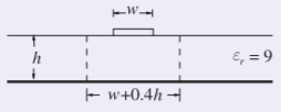
Figure \(\PageIndex{6}\)

Solution

\(h = 2.5\text{ mm},\: w = 1\text{ mm},\: \lambda = \lambda_{0}/\sqrt{\varepsilon_{r}} = \lambda_{0}/3\)

1. The magnetic waveguide model of Figure \(\PageIndex{4}\) can be used in estimating the frequency at which this occurs. The frequency at which the first transverse resonance mode occurs is when there is a full half-wavelength variation of the magnetic field between the magnetic walls, that is, when \(w + 0.4h = \lambda /2=2\text{ mm}\):
   \[\label{eq:5}\frac{\lambda_{0}}{3\cdot 2}=2\text{ mm}⇒\lambda_{0}=12\text{ mm},\quad\text{and so}\quad f_{c,\text{TRAN}}=25\text{ GHz} \]
2. All of the critical multimoding frequencies must be considered here and the minimum taken: for the slab mode, \(f_{c,\text{SLAB}}\) (Equation \(\eqref{eq:1}\)); for the higher-order microstrip mode, fHigh−Microstrip (Equation \(\eqref{eq:2}\)); and for the transverse resonance mode (Equation \(\eqref{eq:5}\)). So the operating frequency range is DC to \(10\text{ GHz}\).

5.4.4 Summary

There are three principal higher-order modes that need to be considered with microstrip transmission lines:

Mode	Critical Frequency
Dielectric (or substrate) mode with discontinuity	Equation \(\eqref{eq:1}\)
Higher order microstrip mode	Equation \(\eqref{eq:2}\)
Transverse resonance mode	Equation \(\eqref{eq:4}\)

Table \(\PageIndex{1}\)

The lowest frequency determines the upper frequency of transmission line operation with a single mode.