6.3: Low Frequency Capacitance Model of Coupled Lines

Last updated
Save as PDF

Page ID: 41292

\( \newcommand{\vecs}[1]{\overset { \scriptstyle \rightharpoonup} {\mathbf{#1}} } \) \( \newcommand{\vecd}[1]{\overset{-\!-\!\rightharpoonup}{\vphantom{a}\smash {#1}}} \)\(\newcommand{\id}{\mathrm{id}}\) \( \newcommand{\Span}{\mathrm{span}}\) \( \newcommand{\kernel}{\mathrm{null}\,}\) \( \newcommand{\range}{\mathrm{range}\,}\) \( \newcommand{\RealPart}{\mathrm{Re}}\) \( \newcommand{\ImaginaryPart}{\mathrm{Im}}\) \( \newcommand{\Argument}{\mathrm{Arg}}\) \( \newcommand{\norm}[1]{\| #1 \|}\) \( \newcommand{\inner}[2]{\langle #1, #2 \rangle}\) \( \newcommand{\Span}{\mathrm{span}}\) \(\newcommand{\id}{\mathrm{id}}\) \( \newcommand{\Span}{\mathrm{span}}\) \( \newcommand{\kernel}{\mathrm{null}\,}\) \( \newcommand{\range}{\mathrm{range}\,}\) \( \newcommand{\RealPart}{\mathrm{Re}}\) \( \newcommand{\ImaginaryPart}{\mathrm{Im}}\) \( \newcommand{\Argument}{\mathrm{Arg}}\) \( \newcommand{\norm}[1]{\| #1 \|}\) \( \newcommand{\inner}[2]{\langle #1, #2 \rangle}\) \( \newcommand{\Span}{\mathrm{span}}\)\(\newcommand{\AA}{\unicode[.8,0]{x212B}}\)

The low-frequency model of a pair of lossless coupled lines comprises only capacitances. A pair of coupled lines, as shown in Figure \(\PageIndex{1}\)(a), has four terminals. At very low frequencies \(V_{1}\) and \(V_{3}\) are identical as are voltages \(V_{2}\) and \(V_{4}\). So the low-frequency model of the pair of coupled lines has just two terminals in addition to ground, as shown in Figure \(\PageIndex{1}\)(b).

The capacitances in Figure \(\PageIndex{1}\)(b) are the shunt capacitance \(C_{1}\) and \(C_{2}\) and the mutual capacitance \(C_{g}\). In the even mode, the voltages at terminals \(1\) and \(2\) are the same so that \(C_{g}\) vanishes, see Figure \(\PageIndex{1}\)(c). In the odd mode, the voltage at terminal \(2\) is the negative of the voltage at terminal \(1\). The result is that there is a virtual ground between the terminals. Now a better circuit model is that shown in Figure \(\PageIndex{1}\)(d). This is where the restriction that the lines are of equal width is used. This assumption places the virtual ground

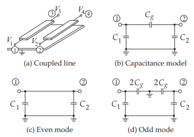
Figure \(\PageIndex{1}\): Very low frequency models of a pair of coupled lines.

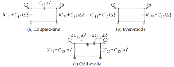
Figure \(\PageIndex{2}\): Low frequency capacitance models of a pair of coupled lines of length \(\Delta\ell\). \(C_{12}\) is negative.

between equal-value capacitances. The symmetrical case is the one of most interest.

To proceed, the capacitance model must be put in the form of per unit length capacitances and put in terms of the elements of a capacitance matrix. The indefinite nodal admittance matrix of the low-frequency coupled-line model of Figure \(\PageIndex{1}\)(b) is

\[\label{eq:1}\mathbf{Y}=\jmath\omega\left[\begin{array}{cc}{C_{1}+C_{g}}&{-C_{g}}\\{-C_{g}}&{C_{2}-C_{g}}\end{array}\right]=\jmath\omega\mathbf{C}\Delta\ell \]

where \(\Delta\ell\) is the length of the coupled lines, and \(C\) is the per unit length capacitance matrix. Thus the low-frequency capacitance model of a pair of coupled lines of length \(\Delta\ell\) and equal width is as shown in Figure \(\PageIndex{2}\)(a). It is found in analysis that \(C_{12}\) is negative.

For symmetrical coupled lines (the strips having the same width) the per unit length even- and odd-mode capacitances, as defined in the definition of odd and even modes in Section 6.2, are

\[\label{eq:2} C_{e}=C_{11}+C_{12}\quad\text{and}\quad C_{o}=C_{11}-C_{12} \]

That is,

\[\label{eq:3}\mathbf{C}=\left[\begin{array}{ll}{C_{11}}&{C_{12}}\\{C_{12}}&{C_{22}}\end{array}\right] =\left[\begin{array}{ll}{\frac{1}{2}(C_{e}+C_{o})}&{\frac{1}{2}(C_{e}-C_{o})}\\{\frac{1}{2}(C_{e}-C_{o})}&{\frac{1}{2}(C_{e}+C_{o})}\end{array}\right] \]