1.8: Frequency domain and k-space descriptions of waves

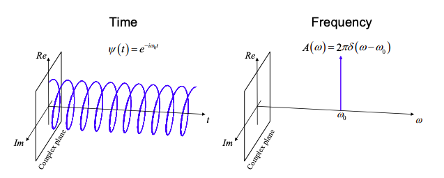
Consider the wavefunction

\[ \psi(t)=ae^{-i\omega_{0}t} \nonumber \]

which describes a wave with amplitude a, intensity \(|a|^{2}\), and phase oscillating in time at angular frequency \(\omega_{0}\). This wave carries two pieces of information, its amplitude and angular frequency.\(^{†}\) Describing the wave in terms of a and \(\omega_{0}\) is known as the frequency domain description. In Figure 1.8.1, we plot the wavefunction in both the time and frequency domains.

In the frequency domain, the wavefunction is described by a delta function at \(\omega_{0}\). Tools for the exact conversion between time and frequency domains will be presented in the next section. Note that, by convention we use a capitalized function (A instead of \(\omega\)) to represent the wavefunction in the frequency domain. Note also that the convention in quantum mechanics is to use a negative sign in the phase when representing the angular frequency \(+\omega_{0}\). This is convenient for describing plane waves of the form \(e^{i(kx-\omega t)}\). But it is exactly opposite to the usual convention in signal analysis (i.e. 6.003). In general, when you see i instead of j for the square root of -1, use this convention in the time and frequency domains.

Figure \(\PageIndex{1}\): Representations of the angular frequency \(\omega_{0}\) in time and frequency domains.

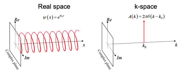
Similarly, consider the wavefunction

\[ \psi(x)=ae^{ik_{0}x} \nonumber \]

which describes a wave with amplitude a, intensity \(|a|^{2}\), and phase oscillating in space with spatial frequency or wavenumber, \(k_{0}\). Again, this wave carries two pieces of information, its amplitude and wavenumber. We can describe this wave in terms of its spatial frequencies in k-space, the equivalent of the frequency domain for spatially oscillating waves. In Figure 1.8.2, we plot the wavefunction in real space and k-space.

Figure \(\PageIndex{2}\): Representations of wavenumber \(k_{0}\) in real space and k-space.

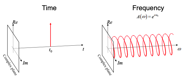
Next, let's consider the wavefunction

\[ A(\omega) = ae^{i\omega t_{0}} \nonumber \]

which describes a wave with amplitude a, intensity \(|a|^{2}\), and phase oscillating in the frequency domain with period \(2\pi/t_{0}\). This wave carries two pieces of information, its amplitude and the time \(t_{0}\). In Figure 1.8.3, we plot the wavefunction in both the time and frequency domains.

Figure \(\PageIndex{3}\): Representations of time \(t_{0}\) in time and frequency domains.

Finally, consider the wavefunction

\[ A(k) = ae^{-ikx_{0}} \nonumber \]

which describes a wave with amplitude a, intensity \(|a|^{2}\), and phase oscillating in k-space with period \(2\pi/x_{0}\). This waves carries two pieces of information, its amplitude and the position \(x_{0}\). In Figure 1.8.4, we plot the wavefunction in both real space and k-space.

Figure \(\PageIndex{4}\): Representations of position \(x_{0}\) in real space and k-space.

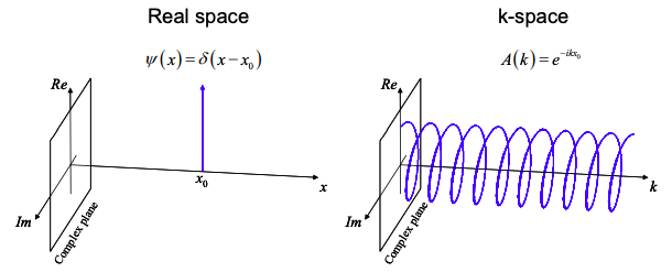
Note that, by convention we use a capitalized function (A instead of \(\psi\)) to represent the wavefunction in the k-space domain.

Observe in Figure 1.8.1-Figure 1.8.4 that a precise definition of both the position in time and the angular frequency of a wave is impossible. A wavefunction with angular frequency of precisely \(\psi_{0}\) is uniformly distributed over all time. Similarly, a wavefunction associated with a precise time \(t_{0}\) contains all angular frequencies.

In real and k-space we also cannot precisely define both the wavenumber and the position. A wavefunction with a wavenumber of precisely \(k_{0}\) is uniformly distributed over all space. Similarly, a wavefunction localized at a precise position \(x_{0}\) contains all wavenumbers.

\(^{†}\) Note the information in any constant phase offset, \(\phi\), as in \(\psi= \text{ exp}[i\omega_{0}t+i\phi]\) can be contained in the amplitude prefactor, i.e. \(\psi= a\text{ exp}[i\omega_{0}t]\), where \(a=\text{exp}[i\phi]\).