1.31: Problems
- Page ID
- 50137
\( \newcommand{\vecs}[1]{\overset { \scriptstyle \rightharpoonup} {\mathbf{#1}} } \)
\( \newcommand{\vecd}[1]{\overset{-\!-\!\rightharpoonup}{\vphantom{a}\smash {#1}}} \)
\( \newcommand{\dsum}{\displaystyle\sum\limits} \)
\( \newcommand{\dint}{\displaystyle\int\limits} \)
\( \newcommand{\dlim}{\displaystyle\lim\limits} \)
\( \newcommand{\id}{\mathrm{id}}\) \( \newcommand{\Span}{\mathrm{span}}\)
( \newcommand{\kernel}{\mathrm{null}\,}\) \( \newcommand{\range}{\mathrm{range}\,}\)
\( \newcommand{\RealPart}{\mathrm{Re}}\) \( \newcommand{\ImaginaryPart}{\mathrm{Im}}\)
\( \newcommand{\Argument}{\mathrm{Arg}}\) \( \newcommand{\norm}[1]{\| #1 \|}\)
\( \newcommand{\inner}[2]{\langle #1, #2 \rangle}\)
\( \newcommand{\Span}{\mathrm{span}}\)
\( \newcommand{\id}{\mathrm{id}}\)
\( \newcommand{\Span}{\mathrm{span}}\)
\( \newcommand{\kernel}{\mathrm{null}\,}\)
\( \newcommand{\range}{\mathrm{range}\,}\)
\( \newcommand{\RealPart}{\mathrm{Re}}\)
\( \newcommand{\ImaginaryPart}{\mathrm{Im}}\)
\( \newcommand{\Argument}{\mathrm{Arg}}\)
\( \newcommand{\norm}[1]{\| #1 \|}\)
\( \newcommand{\inner}[2]{\langle #1, #2 \rangle}\)
\( \newcommand{\Span}{\mathrm{span}}\) \( \newcommand{\AA}{\unicode[.8,0]{x212B}}\)
\( \newcommand{\vectorA}[1]{\vec{#1}} % arrow\)
\( \newcommand{\vectorAt}[1]{\vec{\text{#1}}} % arrow\)
\( \newcommand{\vectorB}[1]{\overset { \scriptstyle \rightharpoonup} {\mathbf{#1}} } \)
\( \newcommand{\vectorC}[1]{\textbf{#1}} \)
\( \newcommand{\vectorD}[1]{\overrightarrow{#1}} \)
\( \newcommand{\vectorDt}[1]{\overrightarrow{\text{#1}}} \)
\( \newcommand{\vectE}[1]{\overset{-\!-\!\rightharpoonup}{\vphantom{a}\smash{\mathbf {#1}}}} \)
\( \newcommand{\vecs}[1]{\overset { \scriptstyle \rightharpoonup} {\mathbf{#1}} } \)
\(\newcommand{\longvect}{\overrightarrow}\)
\( \newcommand{\vecd}[1]{\overset{-\!-\!\rightharpoonup}{\vphantom{a}\smash {#1}}} \)
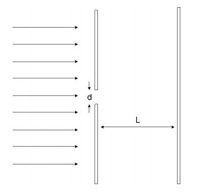
\(\newcommand{\avec}{\mathbf a}\) \(\newcommand{\bvec}{\mathbf b}\) \(\newcommand{\cvec}{\mathbf c}\) \(\newcommand{\dvec}{\mathbf d}\) \(\newcommand{\dtil}{\widetilde{\mathbf d}}\) \(\newcommand{\evec}{\mathbf e}\) \(\newcommand{\fvec}{\mathbf f}\) \(\newcommand{\nvec}{\mathbf n}\) \(\newcommand{\pvec}{\mathbf p}\) \(\newcommand{\qvec}{\mathbf q}\) \(\newcommand{\svec}{\mathbf s}\) \(\newcommand{\tvec}{\mathbf t}\) \(\newcommand{\uvec}{\mathbf u}\) \(\newcommand{\vvec}{\mathbf v}\) \(\newcommand{\wvec}{\mathbf w}\) \(\newcommand{\xvec}{\mathbf x}\) \(\newcommand{\yvec}{\mathbf y}\) \(\newcommand{\zvec}{\mathbf z}\) \(\newcommand{\rvec}{\mathbf r}\) \(\newcommand{\mvec}{\mathbf m}\) \(\newcommand{\zerovec}{\mathbf 0}\) \(\newcommand{\onevec}{\mathbf 1}\) \(\newcommand{\real}{\mathbb R}\) \(\newcommand{\twovec}[2]{\left[\begin{array}{r}#1 \\ #2 \end{array}\right]}\) \(\newcommand{\ctwovec}[2]{\left[\begin{array}{c}#1 \\ #2 \end{array}\right]}\) \(\newcommand{\threevec}[3]{\left[\begin{array}{r}#1 \\ #2 \\ #3 \end{array}\right]}\) \(\newcommand{\cthreevec}[3]{\left[\begin{array}{c}#1 \\ #2 \\ #3 \end{array}\right]}\) \(\newcommand{\fourvec}[4]{\left[\begin{array}{r}#1 \\ #2 \\ #3 \\ #4 \end{array}\right]}\) \(\newcommand{\cfourvec}[4]{\left[\begin{array}{c}#1 \\ #2 \\ #3 \\ #4 \end{array}\right]}\) \(\newcommand{\fivevec}[5]{\left[\begin{array}{r}#1 \\ #2 \\ #3 \\ #4 \\ #5 \\ \end{array}\right]}\) \(\newcommand{\cfivevec}[5]{\left[\begin{array}{c}#1 \\ #2 \\ #3 \\ #4 \\ #5 \\ \end{array}\right]}\) \(\newcommand{\mattwo}[4]{\left[\begin{array}{rr}#1 \amp #2 \\ #3 \amp #4 \\ \end{array}\right]}\) \(\newcommand{\laspan}[1]{\text{Span}\{#1\}}\) \(\newcommand{\bcal}{\cal B}\) \(\newcommand{\ccal}{\cal C}\) \(\newcommand{\scal}{\cal S}\) \(\newcommand{\wcal}{\cal W}\) \(\newcommand{\ecal}{\cal E}\) \(\newcommand{\coords}[2]{\left\{#1\right\}_{#2}}\) \(\newcommand{\gray}[1]{\color{gray}{#1}}\) \(\newcommand{\lgray}[1]{\color{lightgray}{#1}}\) \(\newcommand{\rank}{\operatorname{rank}}\) \(\newcommand{\row}{\text{Row}}\) \(\newcommand{\col}{\text{Col}}\) \(\renewcommand{\row}{\text{Row}}\) \(\newcommand{\nul}{\text{Nul}}\) \(\newcommand{\var}{\text{Var}}\) \(\newcommand{\corr}{\text{corr}}\) \(\newcommand{\len}[1]{\left|#1\right|}\) \(\newcommand{\bbar}{\overline{\bvec}}\) \(\newcommand{\bhat}{\widehat{\bvec}}\) \(\newcommand{\bperp}{\bvec^\perp}\) \(\newcommand{\xhat}{\widehat{\xvec}}\) \(\newcommand{\vhat}{\widehat{\vvec}}\) \(\newcommand{\uhat}{\widehat{\uvec}}\) \(\newcommand{\what}{\widehat{\wvec}}\) \(\newcommand{\Sighat}{\widehat{\Sigma}}\) \(\newcommand{\lt}{<}\) \(\newcommand{\gt}{>}\) \(\newcommand{\amp}{&}\) \(\definecolor{fillinmathshade}{gray}{0.9}\)1. Suppose we fire electrons through a single slit with width d. At the viewing screen behind the aperture, the electrons will form a pattern. Derive and sketch the expression for the intensity at the viewing screen. State all necessary assumptions.

How does this pattern differ from the pattern with two slits discussed in class?
2. Compare the different patterns at the viewing screen with d = 20Å and L = 100nm for fired electrons with wavelengths of 10Å, 100Å, and 1000Å. Explain.
3. Show that a shift in the position of a wavepacket by \(x_{0}\) is equivalent to multiplying the k-space representation by \(\text{exp}[-ikx_{0}]\). Also, show that a shift in the k-space representation by \(k_{0}\) is equivalent to multiplying the position of the wavepacket by \(\text{exp}[-ik_{0}x]\). Show that similar relations hold for shifts in time and frequency.
4. Find \(|F(\omega)|^{2}\) where \(F(\omega)\) is the Fourier Transform of an exponential decay:
\[ F(\omega)= \mathcal{F}[e^{-at}u(t)] \nonumber \]
where u(t) is the unit step function.
5. Show that if
\[ (\Delta x)^{2} = \langle x^{2}\rangle - \langle x\rangle^{2} \nonumber \]
then
\[ \Delta x=\sigma \nonumber \]
where
\[ \psi(x)=\text{exp}[-\frac{1}{4}\frac{(x-x_{0})^{2}}{\sigma^{2}}] \nonumber \]
6. Show the following:
(a) \( \langle k\rangle=\frac{\langle A|k| A\rangle}{\langle A \mid A\rangle}=\frac{\left\langle\psi\left|-i \frac{d}{d x}\right| \psi\right\rangle}{\langle\psi \mid \psi\rangle} \)
(b) \( \langle \omega\rangle=\frac{\langle A|\omega| A\rangle}{\langle A \mid A\rangle}=\frac{\left\langle\psi\left|i \frac{d}{d t}\right| \psi\right\rangle}{\langle\psi \mid \psi\rangle} \)
7. A free particle is confined to move along the x-axis. At time t=0 the wave function is given by
\[ \psi(x, t=0)=\left\{\begin{array}{cc}
\frac{1}{\sqrt{L}} e^{i k_{0} x} & \frac{-L}{2} \leq x \leq \frac{L}{2} \\
0 & \text { otherwise }
\end{array}\right. \nonumber \]
(a) What is the most probable value of momentum?
(b) What are the least probable values of momentum?
(c) Make a rough sketch of the wave function in k-space, A(k, t=0).
8. The commutator of two operators \(\hat{A}\) and \(\hat{B}\) is defined as
\[ [\hat{A},\hat{B}]=\hat{A}\hat{B}-\hat{B}\hat{A} \nonumber \]
Evaluate the following commutators:
(a) \([\hat{x},\hat{x}^{2}]\)
(b) \([\hat{p},\hat{p}^{2}]\)
(c) \([\hat{x}^{2},\hat{p}^{2}]\)
(d) \([\hat{x}\hat{p},\hat{p}\hat{x}]\)
9. Consider the wavefunction
\[ \psi(x)=\exp \left[-\frac{1}{2} \frac{x^{2}}{\sigma^{2}}(1+i C)\right] \nonumber \]
Show that
\[ \left|\sigma_{x}\right|\left|\sigma_{k}\right| \geq \frac{1}{2} \sqrt{1+C^{2}} \nonumber \]
(Hint: Show that \( |\sigma_{k}^{2}|=\frac{\langle \psi|-\frac{d^{2}}{dx^{2}}|\psi \rangle}{\langle \psi|\psi \rangle} \)
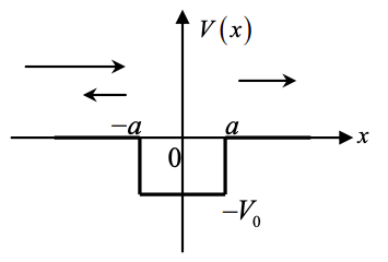
10. For the finite square well shown below, calculate the reflection and transmission coefficients (E > 0).

11. Consider an electron in the ground state of an infinite square well of width L. What is the expectation value of its velocity? What is the expectation value of its kinetic energy? Is there a conflict between your results?
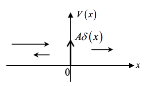
12. Derive the reflection and transmission coefficients for the potential \(V(x)=A\delta(x)\), where A>0.

One method to solve is by taking the Schrödinger equation with \(V(x)=A\delta(x)\)
\[ -\frac{\hbar^{2}}{2 m} \frac{\partial^{2} \psi(x)}{\partial x^{2}}+A \delta(x) \psi(x)=E \psi(x) \nonumber \]
and integrating both sides from \(-\epsilon\) to \(\epsilon\) for \(\epsilon\) very small to get the constraint
\[ -\frac{\hbar^{2}}{2 m} \int_{-\varepsilon}^{+\varepsilon} \frac{\partial^{2} \psi(x)}{\partial x^{2}} d x+A \psi(0) \simeq 2 \varepsilon E \psi(0) \simeq 0 \nonumber \]
\( \left.\Rightarrow \frac{d \psi}{d x}\right|_{x=\varepsilon}-\left.\frac{d \psi}{d x}\right|_{x=-\varepsilon}=\frac{2 m A}{\hbar^{2}} \psi(0) \)
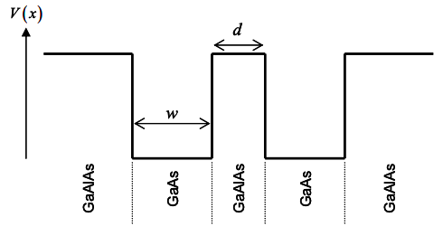
13. Consider two quantum wells each with width w separated by distance d.

(a) From your understanding of wavefunctions for a particle in a box, plot the approximate probability density for each of the two lowest energy modes for this system when the two quantum wells are isolated from each other.
(b) Plot the two lowest energy modes when the two quantum wells are brought close to each other such that d\llw?
(c) Next we wish to take a thin slice of another material and insert it in the structure above (where d\llw) to kill one of the two modes of part (b) but leave the other unaffected. How would you choose the material (compared to the materials already present in the structure), and where should this new material be placed?

