2.7: The Schrödinger Equation in Higher Dimensions
- Page ID
- 50022

Analyzing quantum wells and bulk materials requires that we solve the Schrödinger Equation in 2-d and 3-d. The equation in 1-d
\[ \left[-\frac{\hbar^{2}}{2 m} \frac{d^{2}}{d x^{2}}+V(x)\right] \psi(x)=E \psi(x) \nonumber \]
is extended to higher dimensions as follows:
The Kinetic Energy operator
In 1-d
\[ \hat{T}=\frac{\hat{p}_{x}^{2}}{2m} \nonumber \]
Now, the magnitude of the momentum in 3-d can be written
\[ |\textbf{p}|^{2} = p_{x}^{2}+p_{y}^{2}+p_{z}^{2} \nonumber \]
Where \(p_{x}\), \(p_{y}\) and \(p_{z}\) are the components of momentum on the x, y and z axes, respectively. It follows that in 3-d
\[ \hat{T}=\frac{\hat{p}_{x}^{2}}{2m}+\frac{\hat{p}_{y}^{2}}{2m}+\dfrac{\hat{p}_{z}^{2}}{2m} = -\frac{\hbar^{2}}{2m}\left(\frac{d^{2}}{dx^{2}}+\frac{d^{2}}{dy^{2}}+\frac{d^{2}}{dz^{2}}\right) \nonumber \]
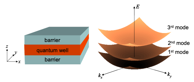
Separable Potential – Quantum Well
A quantum well is shown in Figure 2.6.2(a). We will assume that the potential can be separated into x, y, and z dependent terms
\[ V(x,y,z)=V_{x}(x)+V_{y}(y)+V_{z}(z) \nonumber \]
For example, a quantum well potential is given by
\[ V_{x}(x) = 0 \nonumber \]
\( V_{y}(y) = 0 \)
\( V_{z}(z) = 0 \)
where in the infinite square well approximation \(V_{0} \rightarrow \infty\), and u is the unit step function.
For potentials of this form the Schrödinger Equation can be separated:
\[ {\left[-\frac{\hbar^{2}}{2 m} \frac{d^{2}}{d x^{2}}+V_{x}(x)\right] \psi(x, y, z)+\left[-\frac{\hbar^{2}}{2 m} \frac{d^{2}}{d y^{2}}+V_{y}(y)\right] \psi(x, y, z)} +\left[-\frac{\hbar^{2}}{2 m} \frac{d^{2}}{d z^{2}}+V_{z}(z)\right] \psi(x, y, z)=\left(E_{x}+E_{y}+E_{z}\right) \psi(x, y, z) \nonumber \]
The wavefunction can also be separated
\[ \psi(x,y,z) = \psi_{x}(x)\psi_{y}(y)\psi_{z}(z) \nonumber \]
From Equations 1.28.1 and 1.28.2, the solutions to the infinite quantum well potential are
\[ \psi(x, y, z)=\psi_{x}(x) \psi_{y}(y) \psi_{z}(z)=\sqrt{\frac{2}{L}} \sin \left(n \frac{\pi z}{L}\right) \cdot \exp \left[i k_{x} x\right] \cdot \exp \left[i k_{y} y\right] \nonumber \]
with
\[ E =E_{x}+E_{y}+E_{z} = \frac{\hbar^{2}k_{x}^{2}}{2m}+\frac{\hbar^{2}k_{y}^{2}}{2m}+\frac{n^{2}\hbar^{2}\pi^{2}}{2mL^{2}} \nonumber \]
This dispersion relation is shown in Figure 2.7.1 for the lowest three modes of the quantum well.
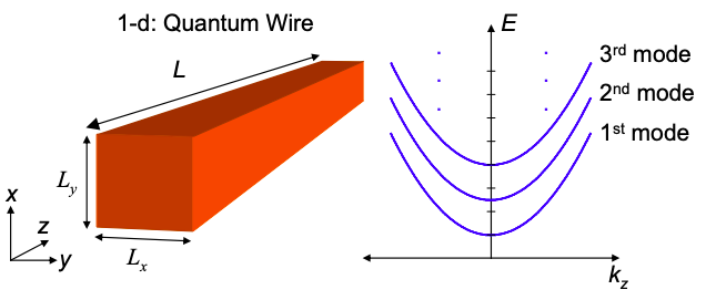
Separable Potential – Quantum Wire
A quantum wire with rectangular cross-section is shown in Figure 2.6.2(b). Again, we will assume that the potential is infinite at the boundaries of the wire:
\[ V(x,y,z) = V_{0}u(-x)+V_{0}u(x-L_{x})+V_{0}u(-y)+V_{0}u(x-L_{y}) \nonumber \]
where \(V_{0} \rightarrow \infty\). The associated wavefunction is confined in the x-y plane and composed of plane waves in the z direction, thus we chose the trial wavefunction
\[ \psi(x,y,z) = \psi(x,y)e^{ik_{z}z} \nonumber \]
Inserting Equation 2.7.12 into the Schrödinger equation gives (for \(0 \leq x \leq L_{x}\) and \(0 \leq y \leq L_{y}\)):
\[ -\frac{\hbar^{2}}{2 m} \frac{d^{2}}{d x^{2}} \psi(x, y)-\frac{\hbar^{2}}{2 m} \frac{d^{2}}{d y^{2}} \psi(x, y)+\frac{\hbar^{2} k_{z}^{2}}{2 m} \psi(x, y)=E \psi(x, y) \nonumber \]
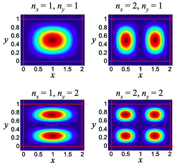
Since the potential goes to infinity at the edges of the wire, \(\psi(x=0)=\psi(x=L_{x})=\psi(y=0)=\psi(y=L_{y})\). Thus, the solution is
\[ \psi(x,y)=\psi_{0}\sin(k_{x}x)\sin(k_{y}y), \nonumber \]
where
\[ k_{x}=\frac{n_{x}\pi}{L_{x}},\ n_{x}=1,2,…,\ k_{y}=1,2,… \nonumber \]
Thus, the constraint in the x- and y-directions defines the discrete energy levels
\[ E_{n_{x}, n_{y}}=\frac{\hbar^{2} \pi^{2}}{2 m}\left(\frac{n_{x}^{2}}{L_{x}^{2}}+\frac{n_{y}^{2}}{L_{y}^{2}}\right), \quad n_{x}, n_{y}=1,2, \ldots \nonumber \]
The total energy is
\[ E_{n_{x}, n_{y}}=\frac{\hbar^{2} \pi^{2}}{2 m}\left(\frac{n_{x}^{2}}{L_{x}^{2}}+\frac{n_{y}^{2}}{L_{y}^{2}}\right) + \frac{\hbar^{2}k_{z}^{2}}{2m}, \quad n_{x}, n_{y}=1,2, \ldots \nonumber \]
This dispersion relation is plotted in Figure 2.7.3 for the lowest three modes.