Engineering LibreTexts

2.14: The 3-d DOS- bulk materials with no confinement

  • Page ID
    50144
  • \( \newcommand{\vecs}[1]{\overset { \scriptstyle \rightharpoonup} {\mathbf{#1}} } \) \( \newcommand{\vecd}[1]{\overset{-\!-\!\rightharpoonup}{\vphantom{a}\smash {#1}}} \)\(\newcommand{\id}{\mathrm{id}}\) \( \newcommand{\Span}{\mathrm{span}}\) \( \newcommand{\kernel}{\mathrm{null}\,}\) \( \newcommand{\range}{\mathrm{range}\,}\) \( \newcommand{\RealPart}{\mathrm{Re}}\) \( \newcommand{\ImaginaryPart}{\mathrm{Im}}\) \( \newcommand{\Argument}{\mathrm{Arg}}\) \( \newcommand{\norm}[1]{\| #1 \|}\) \( \newcommand{\inner}[2]{\langle #1, #2 \rangle}\) \( \newcommand{\Span}{\mathrm{span}}\) \(\newcommand{\id}{\mathrm{id}}\) \( \newcommand{\Span}{\mathrm{span}}\) \( \newcommand{\kernel}{\mathrm{null}\,}\) \( \newcommand{\range}{\mathrm{range}\,}\) \( \newcommand{\RealPart}{\mathrm{Re}}\) \( \newcommand{\ImaginaryPart}{\mathrm{Im}}\) \( \newcommand{\Argument}{\mathrm{Arg}}\) \( \newcommand{\norm}[1]{\| #1 \|}\) \( \newcommand{\inner}[2]{\langle #1, #2 \rangle}\) \( \newcommand{\Span}{\mathrm{span}}\)\(\newcommand{\AA}{\unicode[.8,0]{x212B}}\)

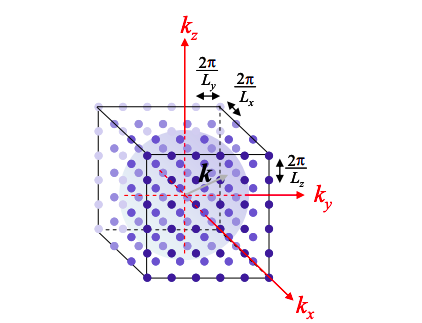
    In 3-d, there is no electron confinement. The only constraint on \(k_{x}\), \(k_{y}\), or \(k_{z}\) are the periodic boundary conditions. We have just shown that if the system has volume \(L_{x}\times L_{y}\times L_{z}\) then each allowed value of k-space occupies a volume of \(2\pi/ L_{x}\times 2\pi/L_{y}\times2\pi/L_{z} = 8\pi^{3}/V\).

    To determine the number of allowed states, we will integrate over all k-space. It is convenient to do this in spherical coordinates. If k is the magnitude of the k vector, the number of modes within a spherical shell of thickness dk is then

    \[ n_{s}(k)dk=2\times \frac{1}{8\pi^{3}/V}\times 4\pi k^{2}dk \nonumber \]

    where \(V = L_{x}\times L_{y}\times L_{z}\), and the factor of two accounts for electron spin. The unconfined wavefunctions within our 3-d box are plane waves in all directions, i.e. the wavefunction could be described by

    \[ \psi(x,y,z) = \psi_{0}e^{ik_{x}x}e^{ik_{y}y}e^{ik_{z}z} \nonumber \]

    Substituting into the Schrödinger Equation gives

    \[ -\frac{\hbar^{2}}{2m} \left( \frac{d^{2}}{dx^{2}}\frac{d^{2}}{dy^{2}} \frac{d^{2}}{dx^{2}}\right) \psi = E \psi \nonumber \]

    Which gives

    \[ \frac{\hbar^{2}}{2m} (k_{x}^{2} + k_{x}^{2}+ k_{x}^{2}) = E \nonumber \]

    Rearranging:

    \[ E = \frac{\hbar^{2}k^{2}}{2m} \nonumber \]

    Screenshot 2021-04-20 at 21.10.15.png
    Figure \(\PageIndex{1}\): Construction used for calculating the DOS for a 3d system.

    Using Equation (2.14.5) to relate E to k gives:

    \[ g(E)dE = \frac{V}{2\pi^{2}}\left( \frac{2m}{\hbar^{2}}\right)^{\frac{3}{2}} \sqrt{E}\ dE \nonumber \]

    where g(E) is the density of states per unit energy.

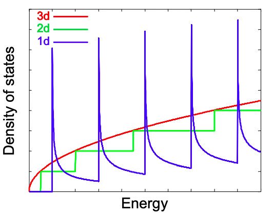
    A comparison of the density of states in 1-d, 2-d and 3-d materials is shown in Figure 2.14.2.

    Screenshot 2021-04-20 at 21.13.53.png
    Figure \(\PageIndex{2}\): Normalized densities of states for bulk materials (3d), quantum wells (2d), and molecular wires (1d).

    This page titled 2.14: The 3-d DOS- bulk materials with no confinement is shared under a CC BY-NC-SA 4.0 license and was authored, remixed, and/or curated by Marc Baldo (MIT OpenCourseWare) via source content that was edited to the style and standards of the LibreTexts platform; a detailed edit history is available upon request.