2.15: Problems

Last updated
Save as PDF

Page ID: 50145

Marc Baldo
Massachusetts Institute of Technology via MIT OpenCourseWare

\( \newcommand{\vecs}[1]{\overset { \scriptstyle \rightharpoonup} {\mathbf{#1}} } \) \( \newcommand{\vecd}[1]{\overset{-\!-\!\rightharpoonup}{\vphantom{a}\smash {#1}}} \)\(\newcommand{\id}{\mathrm{id}}\) \( \newcommand{\Span}{\mathrm{span}}\) \( \newcommand{\kernel}{\mathrm{null}\,}\) \( \newcommand{\range}{\mathrm{range}\,}\) \( \newcommand{\RealPart}{\mathrm{Re}}\) \( \newcommand{\ImaginaryPart}{\mathrm{Im}}\) \( \newcommand{\Argument}{\mathrm{Arg}}\) \( \newcommand{\norm}[1]{\| #1 \|}\) \( \newcommand{\inner}[2]{\langle #1, #2 \rangle}\) \( \newcommand{\Span}{\mathrm{span}}\) \(\newcommand{\id}{\mathrm{id}}\) \( \newcommand{\Span}{\mathrm{span}}\) \( \newcommand{\kernel}{\mathrm{null}\,}\) \( \newcommand{\range}{\mathrm{range}\,}\) \( \newcommand{\RealPart}{\mathrm{Re}}\) \( \newcommand{\ImaginaryPart}{\mathrm{Im}}\) \( \newcommand{\Argument}{\mathrm{Arg}}\) \( \newcommand{\norm}[1]{\| #1 \|}\) \( \newcommand{\inner}[2]{\langle #1, #2 \rangle}\) \( \newcommand{\Span}{\mathrm{span}}\)\(\newcommand{\AA}{\unicode[.8,0]{x212B}}\)

i) Using MATLAB, generate Figure 2.7.2

ii) If \(L_{y} = L_{x} \cdot \sqrt{\frac{3}{5}}\) which mode has a lower energy {\(n_{x}= 3,n_{y} = 1\)} or {\(n_{x}= 2, n_{y} = 2\)}

2. The transistor illustrated below has an oxide ( \(\epsilon = 4\epsilon_{0}\) ) thickness d = 1.2nm and channel depth \(L_{z}\) = 2.5nm. Considering the channel as a quantum well, how many modes are filled when a voltage V=1V is applied to the gate?

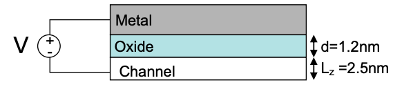
Screenshot 2021-04-20 at 21.19.55.png — Figure \(\PageIndex{28}\): A simple model of a modern transistor.

Hint: calculate the charge in the channel using the expression for a parallel plate capacitor.

3. A particular conductor of length L has the dispersion relation:

\[ \begin{array}{l}
E_{1}(k)=5+2 V \cos (k a) \\
E_{2}(k)=10-2 V \cos (k a)
\end{array},|k|<\frac{\pi}{a} \nonumber \]

where V and a are positive constants.

i) Sketch the dispersion relation.

ii) Calculate the density of states in terms of E, V, and a.

4. In general, the degenerate approximation for the electron distribution function \(f(E,E_{F})\) works when the density of states is large and slowly varying above and below the Fermi level. The non degenerate approximation works best when the density of states at the Fermi level is much smaller than the density of states at higher energies.

Here, we consider these approximations in a Gaussian density of states. The Gaussian varies fairly slowly near its center, but it decreases extremely rapidly in its tails. The electron population in a Gaussian density of states is given by

\[ n = \int^{\infty}_{-\infty} \frac{1}{\sqrt{2\pi\sigma^{2}}} e^{-\frac{1}{2}(E/\sigma)^{2}}f(E,E_{F})dE \nonumber \] ,

where \(f(E,E_{F})\) is the Fermi function. For a particular range of the Fermi level, \(E_{F}\), the electron population may be approximated as:

\[ n \approx \int^{E_{F}}_{-\infty} \frac{1}{\sqrt{2\pi\sigma^{2}}} e^{-\frac{1}{2}(E/\sigma)^{2}}dE \nonumber \]

This is the degenerate limit.

As the Fermi level decreases, the electron population is better calculated in the nondegenerate limit. Derive the minimum Fermi level \(E_{F}\) for the degenerate limit to hold as a function of temperature T and standard deviation \(\sigma\).

Hint: estimate the minimum Fermi level by examining the energetic distribution of electrons in the non-degenerate limit.