8.5: Appendix 4 - Hybrid Orbitals
- Page ID
- 53073
\( \newcommand{\vecs}[1]{\overset { \scriptstyle \rightharpoonup} {\mathbf{#1}} } \)
\( \newcommand{\vecd}[1]{\overset{-\!-\!\rightharpoonup}{\vphantom{a}\smash {#1}}} \)
\( \newcommand{\id}{\mathrm{id}}\) \( \newcommand{\Span}{\mathrm{span}}\)
( \newcommand{\kernel}{\mathrm{null}\,}\) \( \newcommand{\range}{\mathrm{range}\,}\)
\( \newcommand{\RealPart}{\mathrm{Re}}\) \( \newcommand{\ImaginaryPart}{\mathrm{Im}}\)
\( \newcommand{\Argument}{\mathrm{Arg}}\) \( \newcommand{\norm}[1]{\| #1 \|}\)
\( \newcommand{\inner}[2]{\langle #1, #2 \rangle}\)
\( \newcommand{\Span}{\mathrm{span}}\)
\( \newcommand{\id}{\mathrm{id}}\)
\( \newcommand{\Span}{\mathrm{span}}\)
\( \newcommand{\kernel}{\mathrm{null}\,}\)
\( \newcommand{\range}{\mathrm{range}\,}\)
\( \newcommand{\RealPart}{\mathrm{Re}}\)
\( \newcommand{\ImaginaryPart}{\mathrm{Im}}\)
\( \newcommand{\Argument}{\mathrm{Arg}}\)
\( \newcommand{\norm}[1]{\| #1 \|}\)
\( \newcommand{\inner}[2]{\langle #1, #2 \rangle}\)
\( \newcommand{\Span}{\mathrm{span}}\) \( \newcommand{\AA}{\unicode[.8,0]{x212B}}\)
\( \newcommand{\vectorA}[1]{\vec{#1}} % arrow\)
\( \newcommand{\vectorAt}[1]{\vec{\text{#1}}} % arrow\)
\( \newcommand{\vectorB}[1]{\overset { \scriptstyle \rightharpoonup} {\mathbf{#1}} } \)
\( \newcommand{\vectorC}[1]{\textbf{#1}} \)
\( \newcommand{\vectorD}[1]{\overrightarrow{#1}} \)
\( \newcommand{\vectorDt}[1]{\overrightarrow{\text{#1}}} \)
\( \newcommand{\vectE}[1]{\overset{-\!-\!\rightharpoonup}{\vphantom{a}\smash{\mathbf {#1}}}} \)
\( \newcommand{\vecs}[1]{\overset { \scriptstyle \rightharpoonup} {\mathbf{#1}} } \)
\( \newcommand{\vecd}[1]{\overset{-\!-\!\rightharpoonup}{\vphantom{a}\smash {#1}}} \)
\(\newcommand{\avec}{\mathbf a}\) \(\newcommand{\bvec}{\mathbf b}\) \(\newcommand{\cvec}{\mathbf c}\) \(\newcommand{\dvec}{\mathbf d}\) \(\newcommand{\dtil}{\widetilde{\mathbf d}}\) \(\newcommand{\evec}{\mathbf e}\) \(\newcommand{\fvec}{\mathbf f}\) \(\newcommand{\nvec}{\mathbf n}\) \(\newcommand{\pvec}{\mathbf p}\) \(\newcommand{\qvec}{\mathbf q}\) \(\newcommand{\svec}{\mathbf s}\) \(\newcommand{\tvec}{\mathbf t}\) \(\newcommand{\uvec}{\mathbf u}\) \(\newcommand{\vvec}{\mathbf v}\) \(\newcommand{\wvec}{\mathbf w}\) \(\newcommand{\xvec}{\mathbf x}\) \(\newcommand{\yvec}{\mathbf y}\) \(\newcommand{\zvec}{\mathbf z}\) \(\newcommand{\rvec}{\mathbf r}\) \(\newcommand{\mvec}{\mathbf m}\) \(\newcommand{\zerovec}{\mathbf 0}\) \(\newcommand{\onevec}{\mathbf 1}\) \(\newcommand{\real}{\mathbb R}\) \(\newcommand{\twovec}[2]{\left[\begin{array}{r}#1 \\ #2 \end{array}\right]}\) \(\newcommand{\ctwovec}[2]{\left[\begin{array}{c}#1 \\ #2 \end{array}\right]}\) \(\newcommand{\threevec}[3]{\left[\begin{array}{r}#1 \\ #2 \\ #3 \end{array}\right]}\) \(\newcommand{\cthreevec}[3]{\left[\begin{array}{c}#1 \\ #2 \\ #3 \end{array}\right]}\) \(\newcommand{\fourvec}[4]{\left[\begin{array}{r}#1 \\ #2 \\ #3 \\ #4 \end{array}\right]}\) \(\newcommand{\cfourvec}[4]{\left[\begin{array}{c}#1 \\ #2 \\ #3 \\ #4 \end{array}\right]}\) \(\newcommand{\fivevec}[5]{\left[\begin{array}{r}#1 \\ #2 \\ #3 \\ #4 \\ #5 \\ \end{array}\right]}\) \(\newcommand{\cfivevec}[5]{\left[\begin{array}{c}#1 \\ #2 \\ #3 \\ #4 \\ #5 \\ \end{array}\right]}\) \(\newcommand{\mattwo}[4]{\left[\begin{array}{rr}#1 \amp #2 \\ #3 \amp #4 \\ \end{array}\right]}\) \(\newcommand{\laspan}[1]{\text{Span}\{#1\}}\) \(\newcommand{\bcal}{\cal B}\) \(\newcommand{\ccal}{\cal C}\) \(\newcommand{\scal}{\cal S}\) \(\newcommand{\wcal}{\cal W}\) \(\newcommand{\ecal}{\cal E}\) \(\newcommand{\coords}[2]{\left\{#1\right\}_{#2}}\) \(\newcommand{\gray}[1]{\color{gray}{#1}}\) \(\newcommand{\lgray}[1]{\color{lightgray}{#1}}\) \(\newcommand{\rank}{\operatorname{rank}}\) \(\newcommand{\row}{\text{Row}}\) \(\newcommand{\col}{\text{Col}}\) \(\renewcommand{\row}{\text{Row}}\) \(\newcommand{\nul}{\text{Nul}}\) \(\newcommand{\var}{\text{Var}}\) \(\newcommand{\corr}{\text{corr}}\) \(\newcommand{\len}[1]{\left|#1\right|}\) \(\newcommand{\bbar}{\overline{\bvec}}\) \(\newcommand{\bhat}{\widehat{\bvec}}\) \(\newcommand{\bperp}{\bvec^\perp}\) \(\newcommand{\xhat}{\widehat{\xvec}}\) \(\newcommand{\vhat}{\widehat{\vvec}}\) \(\newcommand{\uhat}{\widehat{\uvec}}\) \(\newcommand{\what}{\widehat{\wvec}}\) \(\newcommand{\Sighat}{\widehat{\Sigma}}\) \(\newcommand{\lt}{<}\) \(\newcommand{\gt}{>}\) \(\newcommand{\amp}{&}\) \(\definecolor{fillinmathshade}{gray}{0.9}\)Linear alignment with two neighbors (sp hybridization)
Consider three atoms in a line, as shown in Figure \(\PageIndex{1}\). Arbitrarily we align the atoms with the x-axis.
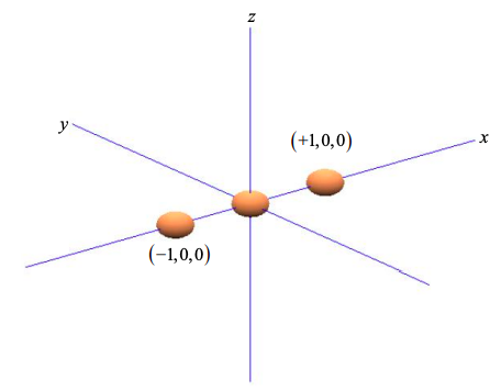
We wish to determine the contribution of the central atom's orbitals to \(\sigma\) bonds. Recall that \(\sigma\) bonds have electron density on the axis between the atoms.
Now, if the basis set consists of s and p orbitals, only \(s\) and \(p_{x}\) orbitals can contribute to \(\sigma\) bonds on the x-axis. \(p_{y}\) and \(p_{z}\) orbitals have zero density on the x-axis and therefore cannot contribute to the \(\sigma\) bonds. They may contribute to \(\pi\) bonds however.
Let's define the symmetry adapted atomic orbitals that contribute to \(\sigma\) bonds generally as:
\[ \phi_{\sigma}=c_{s}\phi_{s}+c_{p_{z}}\phi_{p_{z}} \label{8.5.1} \]
where \(c_{s}\) and \(c_{p_{x}}\) are the weighting coefficients for the \(s\) and \(p_{x}\) orbitals respectively. There are two \(\sigma\) bonds: one to the left, and one to the right. We'll define the two symmetry adapted atomic orbitals that contribute to these \(\sigma\) bonds as \(\phi_{\sigma}^{1}\) and \(\phi_{\sigma}^{2}\) respectively.
The s orbital contributes equally to both symmetry adapted atomic orbitals. i.e.
\[ |c_{s}|^{2} = \frac{1}{2},\ \ \ c_{s} =\frac{1}{\sqrt{2}} \label{8.5.2} \]
Since the \(p_{x}\) orbital is aligned with the x-axis, we can weight the \(p_{x}\) orbital components by the coordinates of the two neighboring atoms at x = +1 and x = -1,
\[ \phi_{\sigma}^{1} = c_{s}\phi_{s} + c_{p}\phi_{p_{x}} \\
\phi_{\sigma}^{2} = c_{s}\phi_{s} - c_{p}\phi_{p_{x}} \label{8.5.3} \]
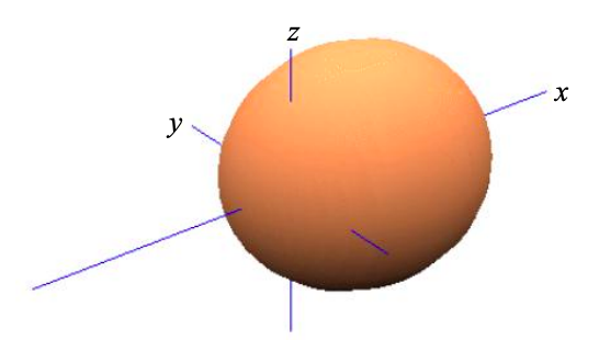
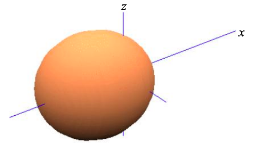
In the first orbital, we are adding the s and \(p_{x}\) orbitals in-phase. Consequently, we have maximum electron density in the positive x-direction. In the second, we are adding the s and \(p_{x}\) orbitals out of phase, yielding a maximum electron density in the negative x-direction.
Normalizing each orbital gives
\[ |c_{p}|^{2} = \frac{1}{2},\ \ \ c_{p} =\sqrt{\frac{1}{2}} \label{8.5.4} \]
Thus, the first symmetry adapted atomic orbital is
\[ \phi_{\sigma}^{1} = \frac{1}{\sqrt{2}}(\phi_{s}+\phi_{p_{x}}) \label{8.5.5} \]
Similarly, the second symmetry adapted atomic orbital is
\[ \phi_{\sigma}^{2} = \frac{1}{\sqrt{2}}(\phi_{s}-\phi_{p_{x}}) \label{8.5.6}. \]
Thus, based purely on symmetry arguments, in a linear chain of atoms it is convenient to re-express the four atomic orbitals s, \(p_{x}\), \(p_{y}\) and \(p_{z}\), as
\[ \phi_{\sigma} = \frac{1}{\sqrt{2}}(\phi_{s} \pm\phi_{p_{x}}) \label{8.5.7}, \]
where \(p_{y}\) and \(p_{z}\) remain unaffected. This is known as sp hybridization since we have combined one s atomic orbital, and one p atomic orbital to create two atomic orbitals that contribute to \(\sigma\) bonds.
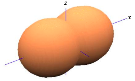
The remaining \(p_{y}\) and \(p_{z}\) atomic orbitals may combine in molecular orbitals with higher energy. The highest occupied molecular orbital (HOMO) is also known as the frontier molecular orbital. In an sp-hybridized material, the frontier molecular orbital will be a linear combination of \(p_{y}\) and \(p_{z}\) atomic orbitals. The frontier molecular orbital is relevant to us, because it more likely than deeper levels to be partially filled. Consequently, conduction is more likely to occur through the HOMO than deeper orbitals.
Now, \(\sigma\) bonds possess electron densities localized between atoms. But \(\pi\) bonds composed of linear combinations of p orbitals can be delocalized along a chain or sheet of atoms. Thus, if the HOMO is a \(\pi\) bond, it is much easier to push an electron through it; we'll see some examples of this in the next section.
Planar alignment with three neighbors (\(sp^{2}\) hybridization)
Consider a central atom with three equispaced neighbors at the points of a triangle; as shown in Figure \(\PageIndex{5}\). Arbitrarily we align the atoms on the x-y plane.
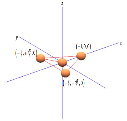
Once again, we wish to determine the contribution of the central atom's orbitals to \(\sigma\) bonds. If the basis set consists of s and p orbitals, only s, \(p_{x}\) and \(p_{y}\) atomic orbitals can contribute to \(\sigma\) bonds in the x-y plane. \(p_{z}\) orbitals can only contribute to \(\pi\) bonds.
Let's define the symmetry adapted atomic orbitals that contribute individually to \(\sigma\) bonds generally as:
\[ \phi_{\sigma} = c_{s}\phi_{s} + c_{p_{x}}\phi_{p_{x}} + c_{p_{y}}\phi_{p_{y}} \label{8.5.8} \]
The s orbital contributes equally to all three symmetry adapted atomic orbitals. i.e.
\[ |c_{s}|^{2} = \frac{1}{3},\ \ \ c_{s} = \frac{1}{\sqrt{3}} \label{8.5.9} \]
Since the \(p_{x}\) orbital is aligned with the x-axis, and \(p_{y}\) with the y-axis, we can weight the p orbital components by the coordinates of the triangle of neighboring atoms
\[ \phi_{\sigma}^{1} = c_{s}\phi_{s} + c_{p} \left( +1\phi_{p_{x}} + 0\phi_{p_{y}} \right) \\
\phi_{\sigma}^{2} = c_{s}\phi_{s} + c_{p} \left( -\frac{1}{2} \phi_{p_{x}} + \frac{\sqrt{3}}{2} \phi_{p_{y}} \right) \\
\phi_{\sigma}^{3} = c_{s}\phi_{s} + c_{p} \left( -\frac{1}{2} \phi_{p_{x}} - \frac{\sqrt{3}}{2} \phi_{p_{y}} \right) \label{8.5.10} \]
Normalizing each orbital gives
\[ |c_{p}|^{2} = \frac{2}{3},\ \ \ c_{p} = \sqrt{\frac{2}{3}} \label{8.5.11} \]
Thus,
\[ \phi_{\sigma}^{1} = \frac{1}{\sqrt{3}} \phi_{s} + \sqrt{\frac{2}{3}} \phi_{p_{x}} + 0 \phi_{p_{y}} \\
\phi_{\sigma}^{2} = \frac{1}{\sqrt{3}} \phi_{s} - \frac{1}{\sqrt{6}} \phi_{p_{x}} + \frac{1}{\sqrt{2}} \phi_{p_{y}} \\
\phi_{\sigma}^{2} = \frac{1}{\sqrt{3}} \phi_{s} - \frac{1}{\sqrt{6}} \phi_{p_{x}} - \frac{1}{\sqrt{2}} \phi_{p_{y}} \nonumber \]
This is known as \(sp^{2}\) hybridization since we have combined one s atomic orbital, and two p atomic orbitals to create three atomic orbitals that contribute individually to \(\sigma\) bonds. The bond angle is 120º.
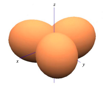
The remaining \(p_{z}\) atomic orbitals will contribute to the frontier molecular orbitals of an \(sp^{2}\) hybridized material; see for example ethene in Figure \(\PageIndex{7}\).
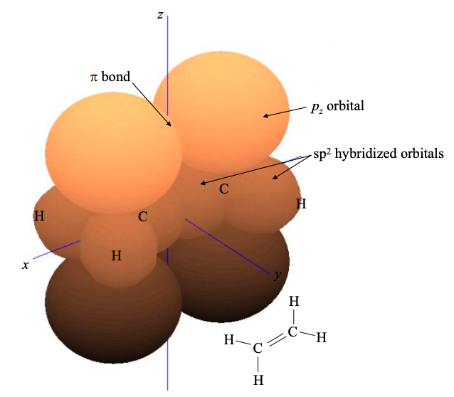
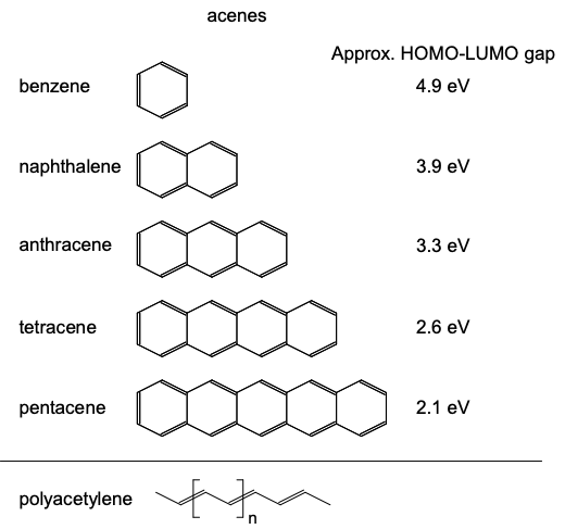
As in the sp hybridized case, electrons in these \(\pi\) molecular orbitals may be delocalized. If electrons are delocalized over several neighboring atoms, then the molecule is said to be conjugated. Another \(sp^{2}\) hybridized material was shown in Figure 6.3.1. This is 1,3- butadiene, a chain of \(4 \times sp^{2}\) hybridized carbon atoms. Note the extensive electron delocalization in the \(\pi\) bonds.
Some archetypal conjugated carbon-based molecules are shown in Figure \(\PageIndex{8}\). In each material the carbon atoms are \(sp^{2}\) hybridized (surrounded by three neighbors at points of an equilateral triangle). Note that another typical characteristic of \(sp^{2}\) hybridized materials is alternating single and double bonds.
Tetrahedral alignment with four neighbors (\(sp^{3}\) hybridization)
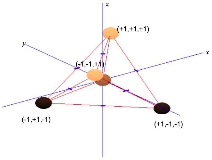
Consider a central atom with four equispaced neighbors. Repulsion between these atoms will push them to the points of a tetrahedron; see Figure \(\PageIndex{9}\).
Now, all atomic orbitals will contribute to \(\sigma\) bonds. There are no \(\pi\) bonds.
Let's define the symmetry adapted atomic orbitals that contribute individually to \(\sigma\) bonds generally as:
\[ \phi_{\sigma} = c_{s}\phi_{s} + c_{p_{x}}\phi_{p_{x}} + c_{p_{y}}\phi_{p_{y}} + c_{p_{z}}\phi_{p_{z}} \label{8.5.13} \]
Once again, the s orbital contributes equally to all four symmetry adapted atomic orbitals. i.e.
\[ |c_{s}|^{2} = \frac{1}{4},\ \ \ c_{s} = \frac{1}{2} \label{8.5.14} \]
Since the \(p_{x}\) orbital is aligned with the x-axis, \(p_{y}\) with the y-axis and \(p_{z}\) with the z-axis, we can weight the p orbital components by the coordinates of the triangle of neighboring atoms
\[ \phi_{\sigma}^{1} = c_{s}\phi_{s} + (+1\phi_{p_{x}}\ +1\phi_{p_{y}}\ +1\phi_{p_{x}}) \\
\phi_{\sigma}^{2} = c_{s}\phi_{s} + (-1\phi_{p_{x}}\ +1\phi_{p_{y}}\ -1\phi_{p_{x}}) \\
\phi_{\sigma}^{3} = c_{s}\phi_{s} + (+1\phi_{p_{x}}\ -1\phi_{p_{y}}\ -1\phi_{p_{x}}) \\
\phi_{\sigma}^{1} = c_{s}\phi_{s} + (-1\phi_{p_{x}}\ -1\phi_{p_{y}}\ -1\phi_{p_{x}}) \label{8.5.15} \]
Normalizing each orbital gives
\[ |c_{p}|^{2} = \frac{1}{4},\ \ \ c_{p} = \frac{1}{2} \label{8.5.16} \]
Thus,
\[ \phi_{\sigma}^{1} = \frac{1}{2}(\phi_{s} + \phi_{p_{x}} + \phi_{p_{y}} + \phi_{p_{z}}) \\
\phi_{\sigma}^{2} = \frac{1}{2}(\phi_{s} - \phi_{p_{x}} + \phi_{p_{y}} - \phi_{p_{z}}) \\
\phi_{\sigma}^{3} = \frac{1}{2}(\phi_{s} + \phi_{p_{x}} - \phi_{p_{y}} - \phi_{p_{z}}) \\
\phi_{\sigma}^{4} = \frac{1}{2}(\phi_{s} - \phi_{p_{x}} - \phi_{p_{y}} - \phi_{p_{z}}) \label{8.5.17} \]
This is known as \(sp^{3}\) hybridization since we have combined one s atomic orbital, and three p atomic orbitals to create four possible atomic orbitals that contribute individually to \(\sigma\) bonds. The bond angle is 109.5º.
