
1.6: Gauss's Law
- Page ID
- 88612

\( \newcommand{\vecs}[1]{\overset { \scriptstyle \rightharpoonup} {\mathbf{#1}} } \)
\( \newcommand{\vecd}[1]{\overset{-\!-\!\rightharpoonup}{\vphantom{a}\smash {#1}}} \)
\( \newcommand{\dsum}{\displaystyle\sum\limits} \)
\( \newcommand{\dint}{\displaystyle\int\limits} \)
\( \newcommand{\dlim}{\displaystyle\lim\limits} \)
\( \newcommand{\id}{\mathrm{id}}\) \( \newcommand{\Span}{\mathrm{span}}\)
( \newcommand{\kernel}{\mathrm{null}\,}\) \( \newcommand{\range}{\mathrm{range}\,}\)
\( \newcommand{\RealPart}{\mathrm{Re}}\) \( \newcommand{\ImaginaryPart}{\mathrm{Im}}\)
\( \newcommand{\Argument}{\mathrm{Arg}}\) \( \newcommand{\norm}[1]{\| #1 \|}\)
\( \newcommand{\inner}[2]{\langle #1, #2 \rangle}\)
\( \newcommand{\Span}{\mathrm{span}}\)
\( \newcommand{\id}{\mathrm{id}}\)
\( \newcommand{\Span}{\mathrm{span}}\)
\( \newcommand{\kernel}{\mathrm{null}\,}\)
\( \newcommand{\range}{\mathrm{range}\,}\)
\( \newcommand{\RealPart}{\mathrm{Re}}\)
\( \newcommand{\ImaginaryPart}{\mathrm{Im}}\)
\( \newcommand{\Argument}{\mathrm{Arg}}\)
\( \newcommand{\norm}[1]{\| #1 \|}\)
\( \newcommand{\inner}[2]{\langle #1, #2 \rangle}\)
\( \newcommand{\Span}{\mathrm{span}}\) \( \newcommand{\AA}{\unicode[.8,0]{x212B}}\)
\( \newcommand{\vectorA}[1]{\vec{#1}} % arrow\)
\( \newcommand{\vectorAt}[1]{\vec{\text{#1}}} % arrow\)
\( \newcommand{\vectorB}[1]{\overset { \scriptstyle \rightharpoonup} {\mathbf{#1}} } \)
\( \newcommand{\vectorC}[1]{\textbf{#1}} \)
\( \newcommand{\vectorD}[1]{\overrightarrow{#1}} \)
\( \newcommand{\vectorDt}[1]{\overrightarrow{\text{#1}}} \)
\( \newcommand{\vectE}[1]{\overset{-\!-\!\rightharpoonup}{\vphantom{a}\smash{\mathbf {#1}}}} \)
\( \newcommand{\vecs}[1]{\overset { \scriptstyle \rightharpoonup} {\mathbf{#1}} } \)
\(\newcommand{\longvect}{\overrightarrow}\)
\( \newcommand{\vecd}[1]{\overset{-\!-\!\rightharpoonup}{\vphantom{a}\smash {#1}}} \)
\(\newcommand{\avec}{\mathbf a}\) \(\newcommand{\bvec}{\mathbf b}\) \(\newcommand{\cvec}{\mathbf c}\) \(\newcommand{\dvec}{\mathbf d}\) \(\newcommand{\dtil}{\widetilde{\mathbf d}}\) \(\newcommand{\evec}{\mathbf e}\) \(\newcommand{\fvec}{\mathbf f}\) \(\newcommand{\nvec}{\mathbf n}\) \(\newcommand{\pvec}{\mathbf p}\) \(\newcommand{\qvec}{\mathbf q}\) \(\newcommand{\svec}{\mathbf s}\) \(\newcommand{\tvec}{\mathbf t}\) \(\newcommand{\uvec}{\mathbf u}\) \(\newcommand{\vvec}{\mathbf v}\) \(\newcommand{\wvec}{\mathbf w}\) \(\newcommand{\xvec}{\mathbf x}\) \(\newcommand{\yvec}{\mathbf y}\) \(\newcommand{\zvec}{\mathbf z}\) \(\newcommand{\rvec}{\mathbf r}\) \(\newcommand{\mvec}{\mathbf m}\) \(\newcommand{\zerovec}{\mathbf 0}\) \(\newcommand{\onevec}{\mathbf 1}\) \(\newcommand{\real}{\mathbb R}\) \(\newcommand{\twovec}[2]{\left[\begin{array}{r}#1 \\ #2 \end{array}\right]}\) \(\newcommand{\ctwovec}[2]{\left[\begin{array}{c}#1 \\ #2 \end{array}\right]}\) \(\newcommand{\threevec}[3]{\left[\begin{array}{r}#1 \\ #2 \\ #3 \end{array}\right]}\) \(\newcommand{\cthreevec}[3]{\left[\begin{array}{c}#1 \\ #2 \\ #3 \end{array}\right]}\) \(\newcommand{\fourvec}[4]{\left[\begin{array}{r}#1 \\ #2 \\ #3 \\ #4 \end{array}\right]}\) \(\newcommand{\cfourvec}[4]{\left[\begin{array}{c}#1 \\ #2 \\ #3 \\ #4 \end{array}\right]}\) \(\newcommand{\fivevec}[5]{\left[\begin{array}{r}#1 \\ #2 \\ #3 \\ #4 \\ #5 \\ \end{array}\right]}\) \(\newcommand{\cfivevec}[5]{\left[\begin{array}{c}#1 \\ #2 \\ #3 \\ #4 \\ #5 \\ \end{array}\right]}\) \(\newcommand{\mattwo}[4]{\left[\begin{array}{rr}#1 \amp #2 \\ #3 \amp #4 \\ \end{array}\right]}\) \(\newcommand{\laspan}[1]{\text{Span}\{#1\}}\) \(\newcommand{\bcal}{\cal B}\) \(\newcommand{\ccal}{\cal C}\) \(\newcommand{\scal}{\cal S}\) \(\newcommand{\wcal}{\cal W}\) \(\newcommand{\ecal}{\cal E}\) \(\newcommand{\coords}[2]{\left\{#1\right\}_{#2}}\) \(\newcommand{\gray}[1]{\color{gray}{#1}}\) \(\newcommand{\lgray}[1]{\color{lightgray}{#1}}\) \(\newcommand{\rank}{\operatorname{rank}}\) \(\newcommand{\row}{\text{Row}}\) \(\newcommand{\col}{\text{Col}}\) \(\renewcommand{\row}{\text{Row}}\) \(\newcommand{\nul}{\text{Nul}}\) \(\newcommand{\var}{\text{Var}}\) \(\newcommand{\corr}{\text{corr}}\) \(\newcommand{\len}[1]{\left|#1\right|}\) \(\newcommand{\bbar}{\overline{\bvec}}\) \(\newcommand{\bhat}{\widehat{\bvec}}\) \(\newcommand{\bperp}{\bvec^\perp}\) \(\newcommand{\xhat}{\widehat{\xvec}}\) \(\newcommand{\vhat}{\widehat{\vvec}}\) \(\newcommand{\uhat}{\widehat{\uvec}}\) \(\newcommand{\what}{\widehat{\wvec}}\) \(\newcommand{\Sighat}{\widehat{\Sigma}}\) \(\newcommand{\lt}{<}\) \(\newcommand{\gt}{>}\) \(\newcommand{\amp}{&}\) \(\definecolor{fillinmathshade}{gray}{0.9}\)Now we have to review some field theory. We will be using fields from time to time in this course, and when we need some aspect of field theory, we will introduce what we need at that point. This seems to make more sense than spending several weeks talking about a lot of abstract theory without seeing how or why it can be useful.
The first thing we need to remember is Gauss's Law. Gauss's Law, like most of the fundamental laws of electromagnetism comes not from first principle, but rather from empirical observation and attempts to match experiments with some kind of self-consistent mathematical framework. Gauss's Law states that: \[\begin{array}{l} \oint\limits_{s,} D \ dS &= \ Q_{\text{encl}} \\ &= \ \oint \limits_{v,} \rho (v) \ dV \end{array} \nonumber \]
where \(D\) is the electric displacement vector, which is related to the electric field vector, \(E\), by the relationship \(D = \varepsilon E\). \(\varepsilon\) is called the dielectric constant. In silicon it has a value of \(1.1 \times 10^{-12} \ \frac{\mathrm{F}}{\mathrm{cm}}\). (Note that \(D\) must have units of \(\frac{\mathrm{Coulombs}}{\mathrm{cm}^{2}}\) to have everything work out okay.) \(Q_{\mathrm{encl}}\) is the total amount of charge enclosed in the volume \(V\), which is obtained by doing a volume integral of the charge density \(\rho (v)\).
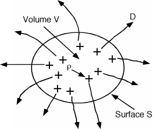
Equation \(\PageIndex{1}\) just says that if you add up the surface integral of the displacement vector \(D\) over a closed surface \(S\), what you get is the sum of the total charge enclosed by that surface. Useful as it is, the integral form of Gauss's Law, (which is what Equation \(\PageIndex{1}\) is) will not help us much in understanding the details of the depletion region. We will have to convert this equation to its differential form. We do this by first shrinking down the volume \(V\) until we can treat the charge density \(\rho (v)\) as a constant \(\rho\), and replace the volume integral with a simple product. Since we are making \(V\) small, let's call it \(\Delta (V)\) to remind us that we are talking about just a small quantity. \[\oint\limits_{\Delta (v),} \rho (v) \ dV \rightarrow \rho \Delta (v) \nonumber \]
And thus, Gauss' Law becomes: \[\begin{array}{l} \oint\limits_{s,} D \ dS &= \varepsilon \oint\limits_{s,} E \ dS \\ &= \rho \Delta (V) \end{array} \nonumber \] or \[\frac{1}{\Delta V} \left(\oint\limits_{s,} E \ dS\right) = \frac{\rho}{\varepsilon} \nonumber \]
Now, by definition the limit of the left hand side of Equation \(\PageIndex{4}\) as \(\Delta (V) \rightarrow 0\) is known as the divergence of the vector \(\mathbf{E}\), or \(\mathrm{div} \mathbf{E}\). Thus we have \[\lim_{\Delta (V) \rightarrow 0} \frac{1}{\Delta (V)} \left(\oint\limits_{s,} E \ dS\right) = \mathrm{div} (\mathbf{E}) = \frac{\rho}{\varepsilon} \nonumber \] Note what this says about the divergence. The divergence of the vector \(\mathbf{E}\) is the limit of the surface integral of \(\mathbf{E}\) over a volume \(V\), normalized by the volume itself, as the volume shrinks to zero. I like to think of as a kind of "point surface integral" of the vector \(\mathbf{E}\).
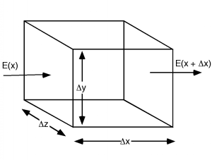
If \(\mathbf{E}\) only varies in one dimension, which is what we are working with right now, the expression for the divergence is particularly simple. It is easy to work out what it is from a simple picture. Looking at Figure \(\PageIndex{2}\) we see that if \(\mathbf{E}\) is only pointed along one direction (let's say \(x\)) and is only a function of \(x\), then the surface integral of \(\mathbf{E}\) over the volume \(\Delta (V) = \Delta (x) \Delta (y) \Delta (x)\) is particularly easy to calculate. \[\oint\limits_{s,} E \ dS = \mathbf{E} (x+\Delta (x)) \Delta (y) \Delta (z) - \mathbf{E}(x) \Delta (y) \Delta (z) \nonumber \]
We remember that the surface integral is defined as being positive for an outward pointing vector and negative for one which points into the volume enclosed by the surface. Now we use the definition of the divergence \[\begin{array}{l} \mathrm{div} (\mathbf{E}) &= \lim_{\Delta (V) \rightarrow 0} \frac{1}{\Delta (V)} \left(\oint\limits_{s,} E \ dS\right) \\ &= \lim_{\Delta (V) \rightarrow 0} \frac{\left(\mathbf{E} (x+\Delta (x)) - \mathbf{E}(x)\right) \Delta (y) \Delta (z)}{\Delta (x) \Delta (y) \Delta (z)} \\ &= \lim_{\Delta (V) \rightarrow 0} \frac{\mathrm{E} (x+\Delta(x)) - \mathrm{E}(x)}{\Delta (x)} \\ &= \frac{\delta \mathbf{E}(x)}{\delta x} \end{array} \nonumber \]
So, we have for the differential form of Gauss' law: \[\frac{\delta \mathbf{E}(x)}{\delta x} = \frac{\rho (x)}{\varepsilon} \nonumber \] Thus, in our case, the rate of change of \(E\) with \(x\), \(\dfrac{d}{dx} (E)\), or the slope of \(E(x)\) is just equal to the charge density, \(\rho (x)\), divided by \(\varepsilon\).