5.7: Bounce Diagrams

Now this new \(V_{2}^{+}\) will head back towards the load and...hmm...things are going to get kind of messy and complicated. Fortunately for us, transmission line engineers came up with a scheme for keeping track of all of the waves bouncing back and forth on the line. The scheme is called a bounce diagram. A bounce diagram consists of a horizontal distance line, which represents distance along the transmission line, and a vertical time axis, which represents time since the battery was first connected to the line. Just to keep things conceptually clear, we usually first start out by showing the line, the battery, the load and a switch, S, which is used to connect the source to the line. It doesn't hurt to make a little sketch like Figure \(\PageIndex{1}\), and write down the length of the line, \(Z_{0}\) and \(v_{p}\), along with the source and load resistances. Now we draw the bounce diagram, which is shown in Figure \(\PageIndex{2}\).

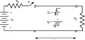Figure \(\PageIndex{1}\): Transient problem

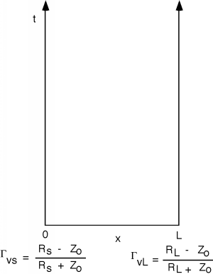Figure \(\PageIndex{2}\): A "bounce diagram"

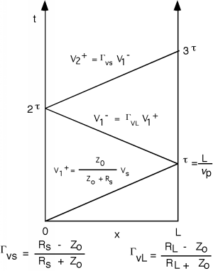
Normally, you would not put the formula for \(\Gamma_{vs}\) and \(\Gamma_{vL}\) by \(x=0\) and \(x=L\) in the diagram, but rather their values. This will become clear when we do an example. The next thing we do is calculate \(V_{1}^{+}\) and draw a straight line on the bounce diagram (nominally at a slope of \(\frac{1}{v_{p}}\)) which will represent the initial signal going down the line. We mark a \(\tau = \frac{L}{v_{p}}\) on the vertical axis to show how long it takes for the wave to reach the end of the line, as shown in Figure \(\PageIndex{3}\).

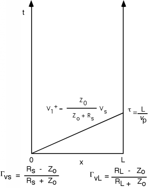Figure \(\PageIndex{3}\): Diagram with first wave

Once the initial wave hits the load, a second, reflected wave \(V_{1}^{-} = \Gamma_{vL} V_{1}^{+}\) is sent back the other way so we add it to the bounce diagram. This is shown in Figure \(\PageIndex{4}\). Since all of the waves move with the same phase velocity, we should be careful to draw all of the lines with the same slope. Note that the time when the reflected wave hits the generator end is a total round trip time of \(2 \tau\). (This simple concept is one which students often forget come test time, so be forewarned!)

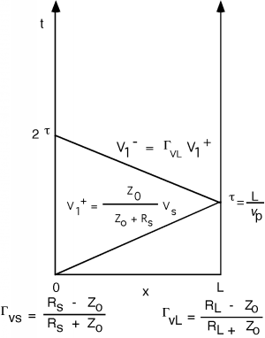Figure \(\PageIndex{4}\): Adding the first reflected wave

We saw that the next thing that happens is that another wave is reflected from the generator, so we add that to the bounce diagram as well. This is shown in Figure \(\PageIndex{5}\).

Figure \(\PageIndex{5}\): The third wave

Finally, one last wave, as we are almost bounced right off the diagram, as shown in Figure \(\PageIndex{6}\)!

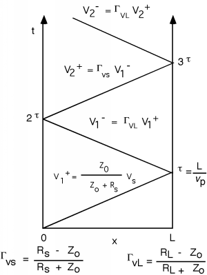Figure \(\PageIndex{6}\): And the fourth wave

OK, so we've got a bounce diagram, so what? Having the diagram is only part of the solution. We still have to see what good they are. Let's do a numerical example, as it is maybe a little more illustrative, and certainly will be easier to write out than all these ratios all the time. We will just pick some typical numbers, and then work out the answers. Let's let \(V_{S} = 40 \mathrm{~V}\), \(R_{S} = 150 \mathrm{~\Omega}\), \(Z_{0} = 50 \mathrm{~\Omega}\), and \(R_{L} = 16.7 \mathrm{~\Omega}\). The line will be 100 meters long, and \(v_{p} = 2 \times 10^{8}\ \frac{\mathrm{m}}{\mathrm{s}}\). The circuit is labeled with these numerical values in Figure \(\PageIndex{7}\).

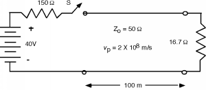Figure \(\PageIndex{7}\): A numerical example

First we calculate the reflection coefficients \[\begin{array}{l} \Gamma_{vL} &= & \dfrac{R_{L} - Z_{0}}{R_{L} + Z_{0}} \\[4pt] &= & \dfrac{16.7 - 50}{16.7 + 50} \\[4pt] &= & -0.50 \end{array}\] and \[\begin{array}{l} \Gamma_{vS} &=& \dfrac{R_{S} - Z_{0}}{R_{S} + Z_{0}} \\[4pt] &=& \dfrac{150-50}{150+50} \\ &=& 0.50 \end{array}\]

The initial voltage signal \(V_{1}^{+}\) is \[\begin{array}{l} V_{1}^{+} &=& \dfrac{50}{50 + 150} \cdot 40 \\[4pt] &=& 10(V) \end{array}\]

and the propagation time is \[\begin{array}{l} \tau &=& \dfrac{L}{v_{p}} \\[4pt] &=& \dfrac{100 \mathrm{~m}}{\left(2 \times 10^{8}\right) \frac{\mathrm{m}}{\mathrm{s}}} \\[4pt] &=& 0.5 \ \mu \mathrm{s} \end{array}\]

So we draw the bounce diagrams seen in Figure \(\PageIndex{8}\).

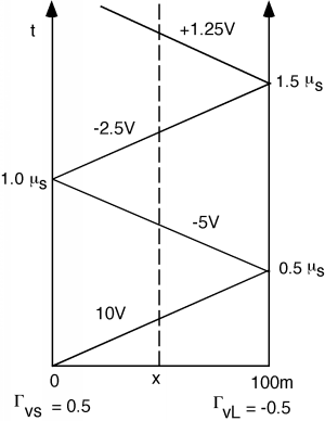Figure \(\PageIndex{8}\): The bounce diagram

Now, here's how we use a bounce diagram, once we have it. Suppose we want to know what \(V(t)\), the voltage as a function of time, would look like halfway down the line. We draw a vertical line at the place we are interested in (the dotted line in Figure \(\PageIndex{8}\)) and then just go up along the line, adding voltage to whatever we had before whenever we cross one of the "bouncing" signal lines. Thus for the line as shown we would have for \(V(t)\) what we see in Figure \(\PageIndex{9}\).

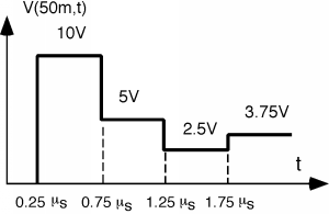Figure \(\PageIndex{9}\): \(V(t)\) at \(50 \mathrm{~m}\) down the line

For the first \(0.25 \ \mu \mathrm{s}\) we have no voltage, because \(V_{1}^{+}\) has not reached the halfway point yet. The voltage then jumps to \(+10 \mathrm{~V}\) when \(V_{1}^{+}\) comes by. It stays like that until the \(V_{1}^{-}\) of \(-5 \mathrm{~V}\) comes by \(0.5 \ \mu \mathrm{s}\) later. The voltage then remains constant at \(5 \mathrm{~V}\) until the \(V_{2}^{+}\) of \(-2.5 \mathrm{~V}\) comes along to drop the total voltage down to only 2.5 volts. When \(V_{2}^{-}\) comes along, it has been switched back to a positive voltage wave by the negative load reflection coefficient, and so now the voltage jumps back up to \(3.75 \mathrm{~V}\). It will keep oscillating back and forth until it finally settles down to some asymptotic value.

What will that asymptotic value be? One approach is to write down the following equation: \[V(x, \infty) = V_{1}^{+} \left(1 + \Gamma_{L} + \Gamma_{L} \Gamma_{S} + \Gamma_{L}{ }^{2} \Gamma_{S} + \ldots\right)\]

which we can re-write as \[V_{1}^{+} \left(1 + \Gamma_{L} \Gamma_{S} + \left(\Gamma_{L}\Gamma_{S}\right)^{2} + \ldots\right) + \Gamma_{L} V_{1}^{+} \left(1 + \Gamma_{L} \Gamma_{S} + \left(\Gamma_{L}\Gamma_{S}\right)^{2} + \ldots\right)\]

Now, remembering the infinite sum relationship \[\sum_{n=0}^{\infty} x^{n} = \frac{1}{1 - x}\]

for \(|x| < 1\) (which is always the case for a reflection coefficient). We can substitute Equation \(\PageIndex{7}\) for the terms inside the parentheses in Equation \(\PageIndex{6}\) and we get \[\begin{array}{l} V(x, \infty) &= V_{1}^{+} \left(\dfrac{1}{1 - \Gamma_{L} \Gamma_{S}} + \dfrac{\Gamma_{L}}{1 - \Gamma_{L} \Gamma_{S}}\right) \\[4pt] &= V_{1}^{+} \dfrac{1 + \Gamma_{L}}{1 - \Gamma_{L}\Gamma_{S}} \end{array}\]

We will leave it as an exercise to the reader to show that if we substitute Equations \(5.6.9\) [link], \(5.6.14\) [link], and finally \(5.6.17\) [link] into Equation \(\PageIndex{8}\) we will eventually get: \[V(x, \infty) = \frac{R_{L}}{R_{L} + R_{S}} V_{S}\]

Look back at Figure \(\PageIndex{1}\) and see if Equation \(\PageIndex{9}\) makes any sense. It should. If we wait long enough, it is reasonable to expect that any "transmission line" effects should go away, and we would be back to the same situation we would have if the line was just some wire connecting the source to the load. In this case, the load resistor and the source resistor would form a voltage divider, and we would expect the voltage across the load to be determined by the voltage divider equation. That's all Equation \(\PageIndex{9}\) is saying!

What do we do if we want, say, the voltage across the load with time? To do this we move up the right-hand side of the bounce diagram, and count voltage waves as we move across them. We start out at zero, of course, and do not see anything until we get to \(0.5 \ \mu \mathrm{s}\). Then we cross the \(10 \mathrm{~V}\) \(V_{1}^{+}\) wave and we cross the \(-5 \mathrm{~V}\) \(V_{1}^{-}\) wave at the same time, so the voltage only goes up to \(+5 \mathrm{~V}\). Likewise, another \(1 \ \mu \mathrm{s}\) later, we cross both the \(-2.5 \mathrm{~V}\) \(V_{2}^{+}\) wave and the \(+1.25 \mathrm{~V}\) \(V_{2}^{-}\) wave, and so the voltage ends up at the \(3.75 \mathrm{~V}\) position as in Figure \(\PageIndex{10}\).

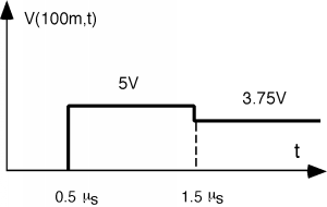Figure \(\PageIndex{10}\): \(V(t)\) across the load

We can also use the bounce diagram to find the voltage as a function of position, for some fixed time \(t_{0}\) as in Figure \(\PageIndex{11}\).

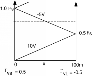Figure \(\PageIndex{11}\): Finding \(V(x)\) at \(t=0.75 \ \mu \mathrm{s}\)

To do this, we draw a horizontal line at the time we are interested in, say \(0.75 \ \mu \mathrm{s}\). Now, for each position \(x\), we go from the bottom of the diagram, up to the horizontal line, adding up voltage as we go. Thus for the example: we get what we see in Figure \(\PageIndex{12}\). For the first half of the line, we cross the \(+10 \mathrm{~V}\) \(V_{1}^{+}\), but that's it. For the second half of the line we cross both the \(+10 \mathrm{~V}\) line as well as the \(-5 \mathrm{~V}\) \(V_{1}^{-}\) wave, and so the voltage drops down to \(5 \mathrm{~V}\).

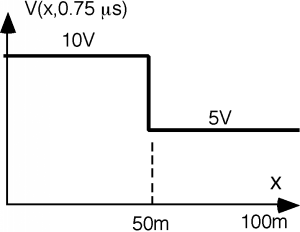Figure \(\PageIndex{12}\): \(V(x)\) at \(t = 0.75 \ \mu \mathrm{s}\)

Of particular interest to many of you will be the way in which a pulse moves down a line and is reflected etc. This is also quite easy to do with a reflection diagram, if we simply break the pulse into two waves, one which has a positive swing at \(t=0\) and another which is a negative going wave at \(t = \tau_{p}\), where \(\tau_{p}\) is the pulse width of the pulse being generated. The way we do this is suggested in Figure \(\PageIndex{13}\). We replace the pulse generator with two battery/switch combinations. The first circuit is just like we have seen so far, with a battery equal to the open circuit pulse height of the generator, and a switch which closes at \(t = 0\). The second circuit has a battery with an amplitude of minus the pulse height, and a switch which closes at \(t = \tau_{p}\), the pulse width of the pulse itself.

Figure \(\PageIndex{13}\): Simulating a pulse with two batteries and two switches

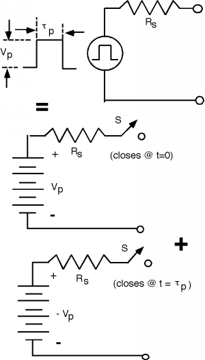
By superposition, we can just add these two generators, one after the other, and see how the pulse goes down the line. Suppose \(V_{p}\) is 10 volts, \(\tau_{p} = 0.25 \ \mu \mathrm{s}\), \(R_{S} = 50 \mathrm{~\Omega}\), \(Z_{0} = 50 \mathrm{~\Omega}\), and \(R_{L} = 25 \mathrm{~\Omega}\). With the numbers, we find that \(V_{1}^{+} = 25 \mathrm{~V}\). \(\Gamma_{vL} = \frac{-1}{3}\), and \(\Gamma_{vS} = 0\). Let's assume that the propagation time on the line is still \(0.5 \ \mu \mathrm{s}\) to get from one end of the line to the other.

We draw the bounce diagram, and launch two waves, one which leaves at \(t=0\), has an amplitude of \(V_{1}^{+} = 5 \mathrm{~V}\). The second wave leaves at a time \(\tau_{p}\) later, and has an amplitude of \(-5 \mathrm{~V}\).

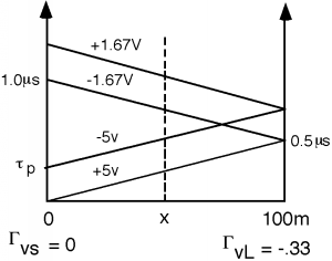Figure \(\PageIndex{14}\): Pulse bounce diagram

Now when we want to see what the voltage as a function of time looks like, we again draw a line up the middle, and add voltages as we cross them. Here we see, again, no voltage until we cross the first wave at \(0.25 \ \mu \mathrm{~s}\), which pops us up to \(+5 \mathrm{~V}\). At a time \(0.25 \ \mu \mathrm{~s}\) later, however, the \(-5 \mathrm{~V}\) wave comes along, and we go back down to zero. At \(t = 0.75 \ \mu \mathrm{~s}\), the reflected \(-1.67 \mathrm{~V}\) pulse comes along, and so we see that. Since the source is matched to the line, \(\Gamma_{vS} = 0\) and so this is the end of the story, as shown in Figure \(\PageIndex{15}\).

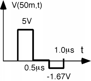Figure \(\PageIndex{15}\): \(V(t)\) halfway down the line

You can get somewhat more interesting waveforms if you go someplace where the two pulses at least partially overlap. Let's look at say, \(x = 87.5 \mathrm{~m}\). Figure \(\PageIndex{16}\) is the bounce diagram.

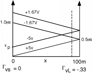Figure \(\PageIndex{16}\): Finding V(t) near the load

And Figure \(\PageIndex{17}\) is the voltage waveform we get.

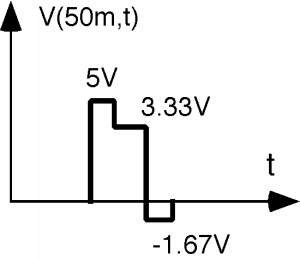Figure \(\PageIndex{17}\): \(V(t)\) near the load

This time the \(1.67 \mathrm{~V}\) pulse gets to us before the \(+5 \mathrm{~V}\) pulse has completely passed, and so we drop from \(5 \mathrm{~V}\) to \(3.33 \mathrm{~V}\). Then, when the \(-5 \mathrm{~V}\) wave goes by, we drop down to \(-1.67 \mathrm{~V}\) for a little while, until the \(+1.67 \mathrm{~V}\) wave comes along to bring us back to zero.